Circular transformations
On this page
Wraparound-aware circular-statistics methods from CircularStatisticsMixin.
Direction (instantaneous)
- static CircularStatisticsMixin.two_point_direction(anterior_loc, posterior_loc)[source]
Calculate directional angles between two body parts.
Computes frame-wise directional angles from posterior to anterior body parts (e.g., tail to nose, nape to head) using arctangent calculations.
It is a validated wrapper around the optimized numba implementation.

See also
For the underlying numba-accelerated implementation, see
simba.mixins.circular_statistics.CircularStatisticsMixin.direction_two_bps()For three-point direction calculation, seesimba.mixins.circular_statistics.CircularStatisticsMixin.three_point_direction()orsimba.mixins.circular_statistics.CircularStatisticsMixin.direction_three_bps()EXPECTED RUNTIMES
FRAMES (MILLIONS)
TIME (S)
TIME (STEV)
1
0.00856
3.80E-04
5
0.03462
0.00238
10
0.06935
0.00038
20
0.13041
0.00238
40
0.2574
0.0026
80
0.5196
0.0038
120
0.79483
0.01722
160
1.05319
0.008966
240
1.70739
0.1392068
ITERATIONS:3
Intel(R) Core(TM) i9-14900KF
- Parameters
anterior_loc (np.ndarray) – 2D array with shape (n_frames, 2) containing [x, y] coordinates for the anterior body part (e.g., nose, head). Must contain non-negative numeric values.
:param np.ndarray posterior_loc : np.ndarray 2D array with shape (n_frames, 2) containing [x, y] coordinates for the posterior body part (e.g., tail base, nape). Must contain non-negative numeric values. :return: 1D array with shape (n_frames,) containing directional angles in degrees [0, 360) for each frame at type float32. Contains NaN values for frames where computation fails. :rtype: np.ndarray
- static CircularStatisticsMixin.three_point_direction(nose_loc, left_ear_loc, right_ear_loc)[source]
Calculate animal heading direction using three anatomical landmarks with input validation.
Computes the mean directional angle of an animal based on nose and ear coordinates using circular statistics. Provides a robust estimate of the animal’s facing direction by calculating individual directional vectors from each ear to the nose, then computing their circular mean to handle angular discontinuities properly.
The function serves as a validated wrapper around the underlying numba-accelerated implementation ensuring input data meet requirements before computation.
See also
For the underlying numba-accelerated implementation, see
simba.mixins.circular_statistics.CircularStatisticsMixin.direction_three_bps(). For two-point direction calculation, seesimba.mixins.circular_statistics.CircularStatisticsMixin.direction_two_bps().
EXPECTED RUNTIMES
FRAMES (MILLIONS)
TIME (S)
TIME (STEV)
1
0.015
1.1406E-06
5
0.0632
0.003
10
0.1206
0.006
20
0.2343
0.016
40
0.4623
0.012
80
0.9052
0.0165
120
1.3953
0.008
160
1.876
0.0532
240
3.1168
0.06966
ITERATIONS:3
Intel(R) Core(TM) i9-14900KF
- Parameters
nose_loc (np.ndarray) – 2D array with shape (n_frames, 2) containing [x, y] pixel coordinates of the nose for each frame. Must contain non-negative numeric values.
left_ear_loc (np.ndarray) – 2D array with shape (n_frames, 2) containing [x, y] pixel coordinates of the left ear for each frame. Must have the same number of frames as nose_loc.
right_ear_loc (np.ndarray) – 2D array with shape (n_frames, 2) containing [x, y] pixel coordinates of the right ear for each frame. Must have the same number of frames as nose_loc.
- Returns
1D array with shape (n_frames,) containing directional angles in degrees [0, 360) for each frame. Contains NaN values for frames where computation fails.
- Return type
np.ndarray
- Example
>>> nose_loc = np.array([[100, 150], [102, 148], [105, 145]], dtype=np.float32)
>>> left_ear_loc = np.array([[95, 160], [97, 158], [100, 155]], dtype=np.float32)
>>> right_ear_loc = np.array([[105, 160], [107, 158], [110, 155]], dtype=np.float32)
>>> directions = CircularStatisticsMixin.direction_three_bps( nose_loc=nose_loc, left_ear_loc=left_ear_loc, right_ear_loc=right_ear_loc)
- static CircularStatisticsMixin.direction_two_bps(anterior_loc, posterior_loc)[source]
Compute directional angle from two body parts using numba acceleration.
Calculates frame-wise directionality between two anatomical landmarks, such as nape to nose or swim bladder to tail. Uses arctangent to determine the heading direction in degrees.
See also
simba.mixins.circular_statistics.CircularStatisticsMixin.direction_three_bps()simba.data_processors.cuda.circular_statistics.direction_from_two_bps()simba.data_processors.cuda.circular_statistics.direction_from_three_bps()- Parameters
anterior_loc (np.ndarray) – Size len(frames) x 2 representing x and y coordinates for first body-part.
posterior_loc (np.ndarray) – Size len(frames) x 2 representing x and y coordinates for second body-part.
- Return np.ndarray
Frame-wise directionality in degrees.
- Example
>>> swim_bladder_loc = np.random.randint(low=0, high=500, size=(50, 2)).astype(np.float32)
>>> tail_loc = np.random.randint(low=0, high=500, size=(50, 2)).astype(np.float32)
>>> CircularStatisticsMixin().direction_two_bps(anterior_loc=swim_bladder_loc, posterior_loc=tail_loc)
- static CircularStatisticsMixin.direction_three_bps(nose_loc, left_ear_loc, right_ear_loc)[source]
Jitted helper to compute the degree angle from three body-parts. Computes the angle in degrees left_ear <-> nose and right_ear_nose and returns the midpoint.
See also
For two-point direction calculation, see
simba.mixins.circular_statistics.CircularStatisticsMixin.direction_two_bps(). For GPU-accelerated implementations, seesimba.data_processors.cuda.circular_statistics.direction_from_two_bps()andsimba.data_processors.cuda.circular_statistics.direction_from_three_bps().- Parameters
nose_loc (ndarray) – 2D array of size len(frames)x2 representing nose coordinates
left_ear_loc (ndarray) – 2D array of size len(frames)x2 representing left ear coordinates
right_ear_loc (ndarray) – 2D array of size len(frames)x2 representing right ear coordinates
- Returns
Array of size nose_loc.shape[0] with direction in degrees.
- Return type
np.ndarray
- Example
>>> nose_loc = np.random.randint(low=0, high=500, size=(50, 2)).astype(np.float32)
>>> left_ear_loc = np.random.randint(low=0, high=500, size=(50, 2)).astype(np.float32)
>>> right_ear_loc = np.random.randint(low=0, high=500, size=(50, 2)).astype(np.float32)
>>> results = CircularStatisticsMixin().direction_three_bps(nose_loc=nose_loc, left_ear_loc=left_ear_loc, right_ear_loc=right_ear_loc)
- static CircularStatisticsMixin.degrees_to_cardinal(data)[source]
Convert degree angles to cardinal direction bucket e.g., 0 -> “N”, 180 -> “S”
Note
To convert cardinal literals to integers, map using
simba.utils.enums.lookups.cardinality_to_integer_lookup(). To convert integers to cardinal literals, map usingsimba.utils.enums.lookups.integer_to_cardinality_lookup().
- Parameters
degree_angles (np.ndarray) – 1d array of degrees. Note: return by
self.head_direction.- Returns
List of strings representing frame-wise cardinality.
- Return type
List[str]
- Example
>>> data = np.array(list(range(0, 405, 45))).astype(np.float32)
>>> CircularStatisticsMixin().degrees_to_cardinal(degree_angles=data)
>>> ['N', 'NE', 'E', 'SE', 'S', 'SW', 'W', 'NW', 'N']
- static CircularStatisticsMixin.sliding_bearing(x, lag, fps)[source]
Calculates the sliding bearing (direction) of movement in degrees for a sequence of 2D points representing a single body-part.
Note
To calculate frame-by-frame bearing, pass fps == 1 and lag == 1.

- Parameters
x (np.ndarray) – An array of shape (n, 2) representing the time-series sequence of 2D points.
lag (float) – The lag time (in seconds) used for calculating the sliding bearing. E.g., if 1, then bearing will be calculated using coordinates in the current frame vs the frame 1s previously.
fps (float) – The sample rate (frames per second) of the sequence.
- Returns
An array containing the sliding bearings (in degrees) for each point in the sequence.
- Return type
np.ndarray
- Example
>>> x = np.array([[10, 10], [20, 10]])
>>> CircularStatisticsMixin.sliding_bearing(x=x, lag=1, fps=1)
>>> [-1. 90.]
Central tendency & dispersion
- static CircularStatisticsMixin.circular_mean(data)[source]
Jitted compute of the circular mean of single sample.
The circular mean is calculated as:
\[\mu = \text{atan2}\left(\frac{1}{N} \sum_{i=1}^{N} \sin(\theta_i), \frac{1}{N} \sum_{i=1}^{N} \cos(\theta_i)\right)\]Where:
\(\theta_i\) are the angles in radians within the sample
\(N\) is the number of samples
\(\mu\) is the circular mean angle
- Parameters
data (np.ndarray) – 1D array of size len(frames) representing angles in degrees.
- Returns
The circular mean of the angles in degrees.
- Return type

See also
simba.data_processors.cuda.circular_statistics.sliding_circular_mean(),simba.mixins.circular_statistics.CircularStatisticsMixin.sliding_circular_mean()- Example
>>> data = np.array([50, 90, 70, 60, 20, 90]).astype(np.float32)
>>> CircularStatisticsMixin().circular_mean(data=data)
>>> 63.737892150878906
- static CircularStatisticsMixin.sliding_circular_mean(data, time_windows, fps)[source]
Compute the circular mean in degrees within sliding temporal windows.

Attention
The returned values represents the angular mean dispersion in the time-window
[current_frame-time_window->current_frame]. -1 is returned whencurrent_frame-time_windowis less than 0.See also
simba.data_processors.cuda.circular_statistics.sliding_circular_mean(),simba.mixins.circular_statistics.CircularStatisticsMixin.circular_mean()- Parameters
data (np.ndarray) – 1d array with feature values in degrees.
time_windows (np.ndarray) – Rolling time-windows as floats in seconds. E.g., [0.2, 0.4, 0.6]
fps (int) – fps of the recorded video
- Returns
Size data.shape[0] x time_windows.shape[0] array
- Return type
np.ndarray
- Example
>>> data = np.random.normal(loc=45, scale=1, size=20).astype(np.float32)
>>> CircularStatisticsMixin().sliding_circular_mean(data=data,time_windows=np.array([0.5, 1.0]), fps=10)
- static CircularStatisticsMixin.circular_std(data)[source]
Jitted compute of the circular standard deviation from a single distribution of angles in degrees.

See also
simba.data_processors.cuda.circular_statistics.sliding_circular_std(),simba.mixins.circular_statistics.CircularStatisticsMixin.sliding_circular_std()\[\sigma_{\text{circular}} = \text{rad2deg}\left(\sqrt{-2 \cdot \log\left(|\text{mean}(\exp(j \cdot \theta))|\right)}\right)\]where \(\theta\) represents the angles in radians
- Parameters
data (ndarray) – 1D array of size len(frames) with angles in degrees
- Returns
The standard deviation of the data sample in degrees.
- Return type
- Example
>>> data = np.array([180, 221, 32, 42, 212, 101, 139, 41, 69, 171, 149, 200]).astype(np.float32)
>>> CircularStatisticsMixin().circular_std(data=data)
>>> 75.03725024504664
- static CircularStatisticsMixin.sliding_circular_std(data, fps, time_windows)[source]
Compute standard deviation of angular data in sliding time windows.

See also
simba.data_processors.cuda.circular_statistics.sliding_circular_std(),simba.mixins.circular_statistics.CircularStatisticsMixin.circular_std()- Parameters
data (ndarray) – 1D array of size len(frames) representing degrees.
time_window (np.ndarray) – Sliding time-window as float in seconds.
fps (int) – fps of the recorded video
- Returns
Size data.shape[0] x time_windows.shape[0] with angular standard deviations in rolling time windows in degrees.
- Return type
np.ndarray
- Example
>>> data = np.array([180, 221, 32, 42, 212, 101, 139, 41, 69, 171, 149, 200]).astype(np.float32)
>>> CircularStatisticsMixin().sliding_circular_std(data=data.astype(np.float32), time_windows=np.array([0.5]), fps=10)
- static CircularStatisticsMixin.mean_resultant_vector_length(data)[source]
Jitted compute of the mean resultant vector length of a single sample. Captures the overall “pull” or “tendency” of the data points towards a central direction on the circle with a range between 0 and 1.
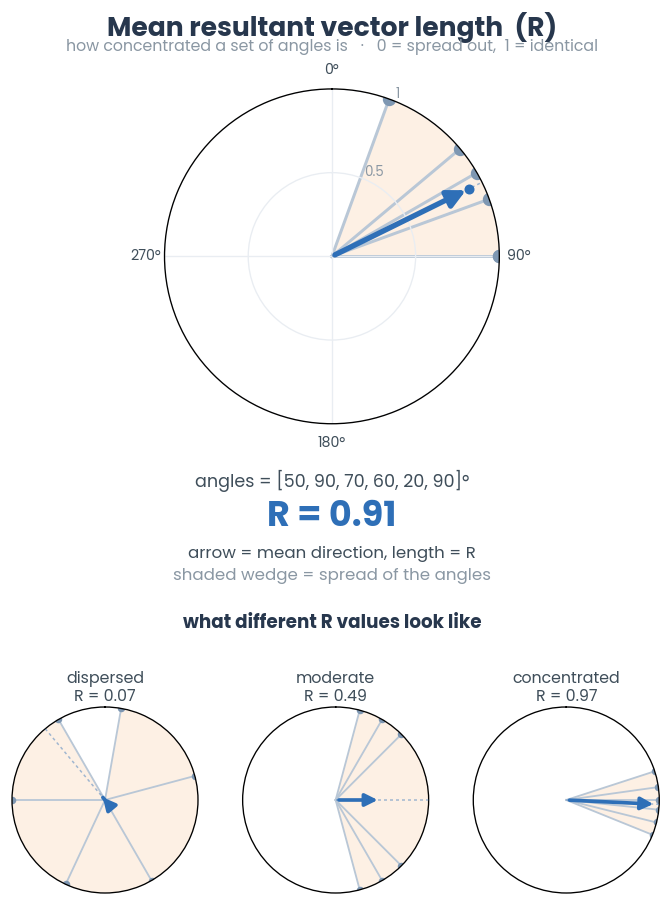 \[R = \frac{{\sqrt{{\sum_{{i=1}}^N \cos(\theta_i - \bar{\theta})^2 + \sum_{{i=1}}^N \sin(\theta_i - \bar{\theta})^2}}}}{{N}}\]
where \(N\) is the number of data points, \(\theta_i\) is the angle of the ith data point, and \(\bar{\theta}\) is the mean angle.
See also
simba.data_processors.cuda.circular_statistics.sliding_resultant_vector_length(),simba.mixins.circular_statistics.CircularStatisticsMixin.sliding_mean_resultant_vector_length()- Parameters
data (np.ndarray) – 1D array of size len(frames) representing angles in degrees.
- Returns
The mean resultant vector of the angles. 1 represents tendency towards a single point. 0 represents no central point.
- Return type
- Example
>>> data = np.array([50, 90, 70, 60, 20, 90]).astype(np.float32)
>>> CircularStatisticsMixin().mean_resultant_vector_length(data=data)
>>> 0.9132277170817057
- static CircularStatisticsMixin.sliding_mean_resultant_vector_length(data, fps, time_windows)[source]
Jitted compute of the mean resultant vector within sliding time window. Captures the overall “pull” or “tendency” of the data points towards a central direction on the circle with a range between 0 and 1.
Attention
The returned values represents resultant vector length in the time-window
[(current_frame-time_window)->current_frame]. -1 is returned wherecurrent_frame-time_windowis less than 0.
See also
simba.data_processors.cuda.circular_statistics.sliding_resultant_vector_length(),simba.mixins.circular_statistics.CircularStatisticsMixin.mean_resultant_vector_length()- Parameters
data (np.ndarray) – 1D array of size len(data) representing degrees.
time_window (np.ndarray) – Rolling time-window as float in seconds.
fps (int) – fps of the recorded video
- Returns
Size len(data) x len(time_windows) representing resultant vector length in the prior
time_window.- Return type
np.ndarray
- Example
>>> data_1, data_2 = np.random.normal(loc=45, scale=1, size=100), np.random.normal(loc=90, scale=45, size=100)
>>> data = np.hstack([data_1, data_2])
>>> CircularStatisticsMixin().sliding_mean_resultant_vector_length(data=data.astype(np.float32),time_windows=np.array([1.0]), fps=10)
- static CircularStatisticsMixin.circular_range(data)[source]
Jitted compute of circular range in degrees. The range is defined as the angular span of the shortest arc that can contain all the data points. A smaller range indicates a more concentrated distribution, while a larger range suggests a more dispersed distribution.
\[\text{Range} = \min \left( 2\pi - \max(\delta \theta_i), \theta_{\text{max}} - \theta_{\text{min}} \right)\]where:
\(\delta \theta_i\) is the difference between consecutive angular data points.
\(\theta_{\text{max}}\) and \(\theta_{\text{min}}\) are the maximum and minimum angles in the data.

See also
simba.data_processors.cuda.circular_statistics.sliding_circular_range(),simba.mixins.circular_statistics.CircularStatisticsMixin.sliding_circular_range()- Parameters
data (ndarray) – 1D array of circular data measured in degrees
- Returns
The circular range in degrees.
- Return type
np.ndarray
- Example
>>> CircularStatisticsMixin().circular_range(np.ndarray([350, 20, 60, 100]))
>>> 110.0
>>> CircularStatisticsMixin().circular_range(np.ndarray([110, 20, 60, 100]))
>>> 90.0
- static CircularStatisticsMixin.sliding_circular_range(data, time_windows, fps)[source]
Jitted compute of sliding circular range for a time series of circular data. The range is defined as the angular span of the shortest arc that can contain all the data points. Measures the circular spread of data within sliding time windows of specified duration.

Note
Output data in the beginning of the series where a full time-window is not satisfied (e.g., first 9 observations when fps equals 10 and time_windows = [1.0], will be populated by
0.See also
simba.data_processors.cuda.circular_statistics.sliding_circular_range(),simba.mixins.circular_statistics.CircularStatisticsMixin.circular_range()- Parameters
data (np.ndarray) – 1D array of circular data measured in degrees
time_windows (np.ndarray) – Size of sliding time window in seconds. E.g., two windows of 0.5s and 1s would be represented as np.array([0.5, 1.0])
fps (int) – Frame-rate of recorded video.
- Returns
Array of size len(sample_1) x len(time_window) with angular ranges in degrees.
- Return type
np.ndarray
- Examples
>>> data = np.array([260, 280, 300, 340, 360, 0, 10, 350, 0, 15]).astype(np.float32)
>>> CircularStatisticsMixin().sliding_circular_range(data=data, time_windows=np.array([0.5]), fps=10)
>>> [[ -1.],[ -1.],[ -1.],[ -1.],[100.],[80],[70],[30],[20],[25]]
Turning direction & angular change
- static CircularStatisticsMixin.preferred_turning_direction(x)[source]
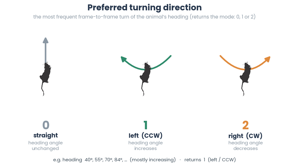
Determines the preferred turning direction from a 1D array of circular directional data.
Note
The input
xcan be created using any of the following methods: -simba.mixins.circular_statistics.CircularStatisticsMixin.direction_two_bps()-simba.data_processors.cuda.circular_statistics.direction_from_two_bps()-simba.data_processors.cuda.circular_statistics.direction_from_three_bps()-simba.mixins.circular_statistics.CircularStatisticsMixin.direction_three_bps()See also
simba.mixins.circular_statistics.CircularStatisticsMixin.rotational_direction(),rotational_direction(),simba.mixins.circular_statistics.CircularStatisticsMixin.sliding_preferred_turning_direction()- Parameters
x (np.ndarray) – 1D array of circular directional data (values between 0 and 360, inclusive). The array represents angular directions measured in degrees.
- Returns
The most frequent turning direction from the input data: - 0: No change in the angular value between consecutive frames. - 1: An increase in the angular value (rotation in the positive direction, counterclockwise). - 2: A decrease in the angular value (rotation in the negative direction, clockwise).
- Return type
- Example
>>> x = np.random.randint(0, 361, (200,))
>>> CircularStatisticsMixin.preferred_turning_direction(x=x)
- static CircularStatisticsMixin.sliding_preferred_turning_direction(x, time_window, sample_rate)[source]
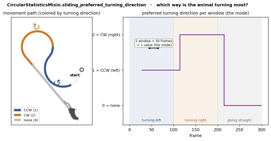
Computes the sliding preferred turning direction over a given time window from a 1D array of circular directional data.
Calculates the most frequent turning direction (mode) within a sliding window of a specified duration.
See also
simba.mixins.circular_statistics.CircularStatisticsMixin.rotational_direction(),rotational_direction(),simba.mixins.circular_statistics.CircularStatisticsMixin.preferred_turning_direction()- Parameters
x (np.ndarray) – A 1D array of circular directional data (values between 0 and 360, inclusive). Each value represents an angular direction in degrees.
time_window (float) – The duration of the sliding window in seconds.
sample_rate (float) – The sampling rate of the data in Hz (samples per second) or FPS (frames per seconds)
- Returns
A 1D array of integers indicating the preferred turning direction for each window: - 0: No change in angular values within the window. - 1: An increase in angular values (counterclockwise rotation). - 2: A decrease in angular values (clockwise rotation). For indices before the first full window, the value is -1.
- Return type
np.ndarray
- Example
>>> x = np.random.randint(0, 361, (213,))
>>> CircularStatisticsMixin.sliding_preferred_turning_direction(x=x, time_window=1, sample_rate=10)
- static CircularStatisticsMixin.rotational_direction(data, stride=1)[source]
Jitted compute of frame-by-frame rotational direction within a 1D timeseries array of angular data.
Note
For the first frame, no rotation is possible so is populated with -1.
Frame-by-frame rotations of 180° degrees are denoted as clockwise rotations.
See also
See
rotational_direction()for GPU acceleration.
The result array contains values: - -1: Indicates no rotation is possible for the first frame. This serves as a placeholder since there is no prior frame to compare to. - 0: Represents no change in the angular value between consecutive frames - 1: Indicates an increase in the angular value (rotation in the positive direction, counterclockwise) - 2: Indicates a decrease in the angular value (rotation in the negative direction, clockwise)
- Parameters
data (np.ndarray) – 1D array of size len(frames) representing degrees.
- Returns
An array of directional indicators.
- Return type
- Example
>>> data = np.array([45, 50, 35, 50, 80, 350, 350, 0 , 180]).astype(np.float32)
>>> CircularStatisticsMixin().rotational_direction(data)
>>> [-1.,  1.,  2.,  1.,  1.,  2.,  0.,  1.,  1.]
- static CircularStatisticsMixin.instantaneous_angular_velocity(data, bin_size)[source]
Jitted compute of absolute angular change in the smallest possible time bin.
Note
If the smallest possible frame-to-frame time-bin in Video 1 is 33ms (recorded at 30fps), and the smallest possible frame-to-frame time-bin in Video 2 is 66ms (recorded at 15fps), we correct for this across recordings using the
bin_sizeargument. E.g., when passing angular data from Video 1 we pass bin_size as2, and when passing angular data for Video 2 we set bin_size to1to allow comparisons of instantaneous angular velocity between Video 1 and Video 2.When current frame minus bin_size results in a negative index, -1 is returned.

- Parameters
data (ndarray) – 1D array of size len(frames) representing degrees.
bin_size (int) – The number of frames prior to compare the current angular velocity against.
- Returns
1D array with instantanous angular velocities according to bin size.
- Return type
np.ndarray
- Example
>>> data = np.array([350, 360, 365, 360]).astype(np.float32)
>>> CircularStatisticsMixin().instantaneous_angular_velocity(data=data, bin_size=1.0)
>>> [-1., 10.00002532, 4.999999, 4.999999]
>>> CircularStatisticsMixin().instantaneous_angular_velocity(data=data, bin_size=2)
>>> [-1., -1., 15.00002432, 0.]
- static CircularStatisticsMixin.sliding_angular_diff(data, time_windows, fps)[source]
Computes the angular difference in the current frame versus N seconds previously. For example, if the current angle is 45 degrees, and the angle N seconds previously was 350 degrees, then the difference is 55 degrees.
Note
Frames where current frame - N seconds prior equal a negative value is populated with
0.Results are returned in rounded nearest integer.

- Parameters
data (ndarray) – 1D array of size len(frames) representing degrees. Can be computed by CircularStatisticsMixin().direction_three_bps or CircularStatisticsMixin().direction_two_bps.
time_window (np.ndarray) – Rolling time-window as float in seconds.
fps (int) – fps of the recorded video
- Example
>>> data = np.array([350, 350, 1, 1]).astype(np.float32)
>>> CircularStatisticsMixin().sliding_angular_diff(data=data, fps=1.0, time_windows=np.array([1.0]))
- static CircularStatisticsMixin.agg_angular_diff_timebins(data, time_windows, fps)[source]
Compute the difference between the median angle in the current time-window versus the previous time window. For example, computes the difference between the mean angle in the first 1s of the video versus the second 1s of the video, the second 1s of the video versus the third 1s of the video, … etc.
Note
The first time-bin of the video cannot be compared against the prior time-bin and is populated with 0.

- Parameters
data (ndarray) – 1D array of size len(frames) representing degrees.
time_window (np.ndarray) – Rolling time-window as float in seconds.
fps (int) – fps of the recorded video
- Example
>>> data = np.random.normal(loc=45, scale=3, size=20).astype(np.float32)
>>> CircularStatisticsMixin().agg_angular_diff_timebins(data=data,time_windows=np.array([1.0]), fps=5.0))
Circular uniformity tests
- static CircularStatisticsMixin.rayleigh(data)[source]
Jitted compute of Rayleigh Z (test of non-uniformity) of single sample of circular data in degrees.
Note
Adapted from
pingouin.circular.circ_rayleighandpycircstat.tests.rayleigh.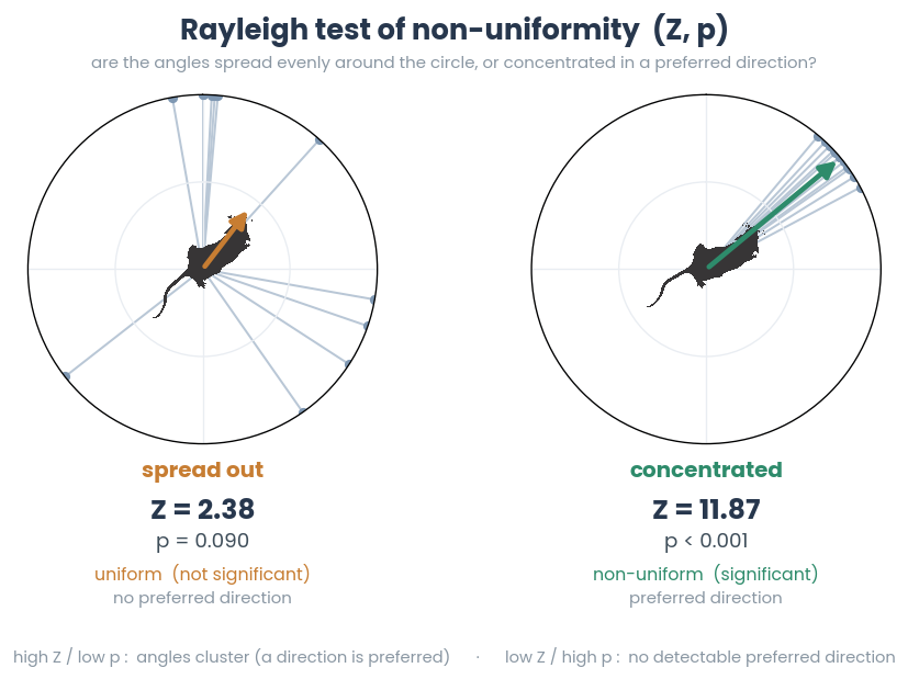
The Rayleigh Z score is calculated as follows:
\[Z = n R^2\]where \(n\) is the sample size and \(R\) is the mean resultant length.
The associated p-value is calculated as follows (note this uses the resultant length \(nR\), not the mean resultant length \(R\)):
\[p = \exp\left(\sqrt{1 + 4n + 4(n^2 - (nR)^2)} - (1 + 2n)\right)\]See also
simba.data_processors.cuda.circular_statistics.sliding_rayleigh_z(),simba.mixins.circular_statistics.CircularStatisticsMixin.sliding_rayleigh_z()- Parameters
data (ndarray) – 1D array of size len(frames) representing degrees.
- Returns
Tuple with Rayleigh Z score and associated probability value.
- Return type
>>> data = np.array([350, 360, 365, 360, 100, 109, 232, 123, 42, 3,4, 145]).astype(np.float32)
>>> CircularStatisticsMixin().rayleigh(data=data)
>>> (2.3845645695246467, 0.09027923051217743)
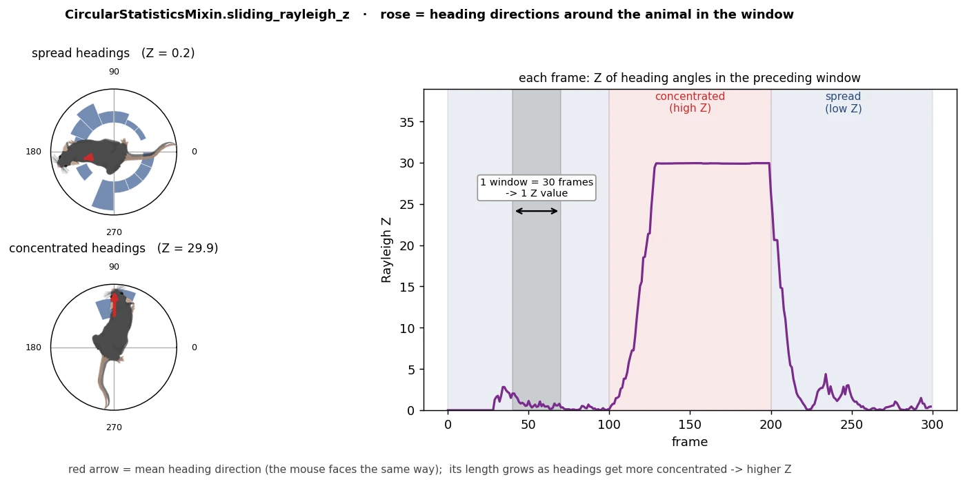
- static CircularStatisticsMixin.sliding_rayleigh_z(data, time_windows, fps)[source]
Jitted compute of Rayleigh Z (test of non-uniformity) of circular data within sliding time-window.
Note
Adapted from
pingouin.circular.circ_rayleighandpycircstat.tests.rayleigh.See also
simba.data_processors.cuda.circular_statistics.sliding_rayleigh_z(),simba.mixins.circular_statistics.CircularStatisticsMixin.rayleigh()- Parameters
data (ndarray) – 1D array of size len(frames) representing degrees.
time_window (np.ndarray) – Rolling time-window as float in seconds. Two windows of 0.5s and 1s would be represented as np.array([0.5, 1.0])
fps (int) – fps of the recorded video
- Returns
Two 2d arrays with the first representing Rayleigh Z scores and second representing associated p values.
- Return type
Tuple[np.ndarray, np.ndarray]
- Example
>>> data = np.random.randint(low=0, high=361, size=(100,)).astype(np.float32)
>>> CircularStatisticsMixin().sliding_rayleigh_z(data=data, time_windows=np.array([0.5, 1.0]), fps=10)
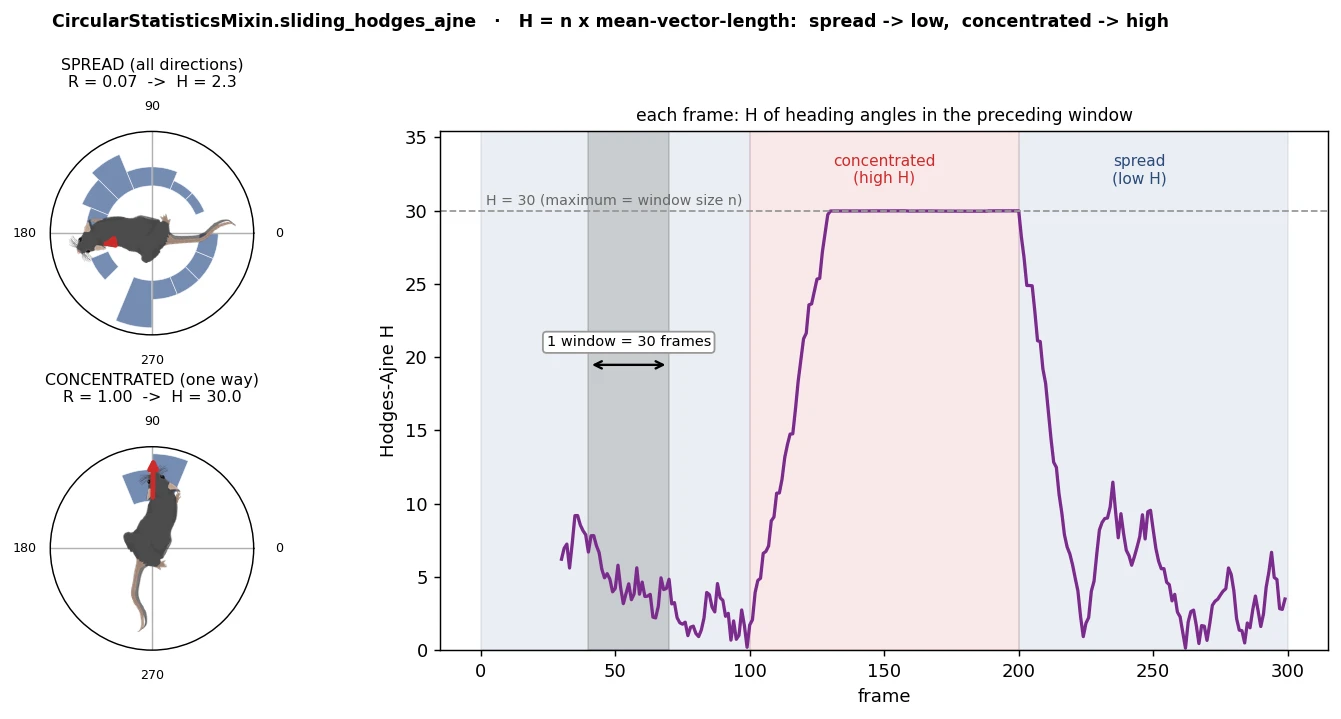
- static CircularStatisticsMixin.sliding_hodges_ajne(data, time_window, fps)[source]
Compute the Hodges-Ajne test statistic for uniformity of circular data within sliding time windows.
The Hodges-Ajne test is a non-parametric test used to assess whether circular data is uniformly distributed. The test statistic measures the concentration of data points around the circle. Lower values indicate more uniform distribution, while higher values suggest clustering or non-uniformity.
Attention
The returned values represent the Hodges-Ajne statistic in the time-window
[(current_frame-time_window)->current_frame]. -1.0 is returned wherecurrent_frame-time_windowis less than 0 (i.e., before the first complete window).The Hodges-Ajne statistic (\(H\)) is calculated as:
\[H = n \cdot (1 - v)\]where:
\(n\) is the number of data points in the sliding window
\(v = 1 - |\text{mean}(\exp(j \cdot \theta))|\) is a measure of dispersion
\(\theta\) are the angles in radians within the window
See also
For computing the Hodges-Ajne statistic on a single sample, see
simba.mixins.circular_statistics.CircularStatisticsMixin.hodges_ajne().- Parameters
- Returns
1D array of size len(data) containing Hodges-Ajne test statistics for each sliding window. Contains -1.0 for frames before the first complete window.
- Return type
np.ndarray
- Example
>>> data = np.random.randint(low=0, high=361, size=(100,)).astype(np.float32)
>>> CircularStatisticsMixin().sliding_hodges_ajne(data=data, time_window=1.0, fps=10)
- static CircularStatisticsMixin.rao_spacing(data)[source]
Jitted compute of Rao’s spacing for angular data.
Computes the uniformity of a circular dataset in degrees. High output values represent concentrated (clustered) angularity with uneven gaps between observations, while low values (near 0) represent evenly-spaced, uniform angularity.
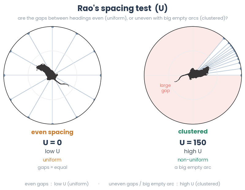
The Rao’s Spacing (\(U\)) is calculated as follows:
\[U = \frac{1}{2} \sum_{i=1}^{N} |l - T_i|\]where \(N\) is the number of data points in the sliding window, \(T_i\) is the spacing between adjacent data points, and \(l\) is the equal angular spacing.
- Parameters
data (ndarray) – 1D array of size len(frames) with data in degrees.
- Returns
Rao’s spacing measure, indicating the dispersion or concentration of angular data points.
- Return type
References
- 1
UCSB.
- Example
>>> data = np.random.randint(0, 360, (5000,)).astype(np.float32)
>>> CircularStatisticsMixin.rao_spacing(data=data)
- static CircularStatisticsMixin.sliding_rao_spacing(data, time_windows, fps)[source]
Jitted compute of the uniformity of a circular dataset in sliding windows.
- Parameters
data (ndarray) – 1D array of size len(frames) representing degrees.
time_window (np.ndarray) – Rolling time-window as float in seconds.
fps (int) – fps of the recorded video
- Return np.ndarray
representing rao-spacing U in every sliding windows [-window:n]

The Rao’s Spacing (\(U\)) is calculated as follows:
\[U = \frac{1}{2} \sum_{i=1}^{N} |l - T_i|\]where \(N\) is the number of data points in the sliding window, \(T_i\) is the spacing between adjacent data points, and \(l\) is the equal angular spacing.
Note
For frames occuring before a complete time window, 0.0 is returned.
References
- 1
UCSB.
- Example
>>> data = np.random.randint(low=0, high=360, size=(500,)).astype(np.float32)
>>> result = CircularStatisticsMixin().sliding_rao_spacing(data=data, time_windows=np.array([0.5, 1.0]), fps=10)
Two-sample tests
- static CircularStatisticsMixin.kuipers_two_sample_test(sample_1, sample_2)[source]
Compute the Kuiper’s two-sample test statistic for circular distributions.
Kuiper’s two-sample test is a non-parametric test used to determine if two samples are drawn from the same circular distribution. It is particularly useful for circular data, such as angles or directions.
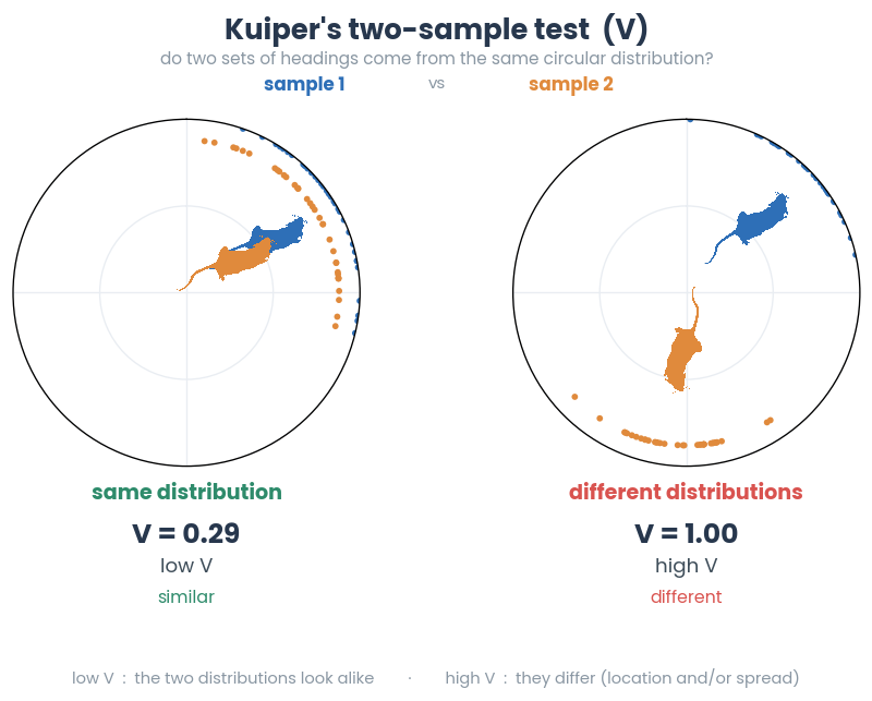
The Kuiper test statistic is calculated as the sum of the maximum positive and negative deviations between the cumulative distribution functions of the two samples:
\[V = \max(F_1(\theta) - F_2(\theta)) + \max(F_2(\theta) - F_1(\theta))\]Where:
\(F_1(\theta)\) and \(F_2(\theta)\) are the empirical cumulative distribution functions (CDFs) of the two circular samples.
\(\theta\) are the sorted angles in the two samples.
Note
Adapted from Kuiper by Anne Archibald.
- Parameters
sample_1 (ndarray) – The first circular sample array in degrees.
sample_2 (ndarray) – The second circular sample array in degrees.
- Returns
Kuiper’s test statistic.
- Return type
- Example
>>> sample_1, sample_2 = np.random.normal(loc=45, scale=1, size=100).astype(np.float32), np.random.normal(loc=180, scale=20, size=100).astype(np.float32)
>>> CircularStatisticsMixin().kuipers_two_sample_test(sample_1=sample_1, sample_2=sample_2)
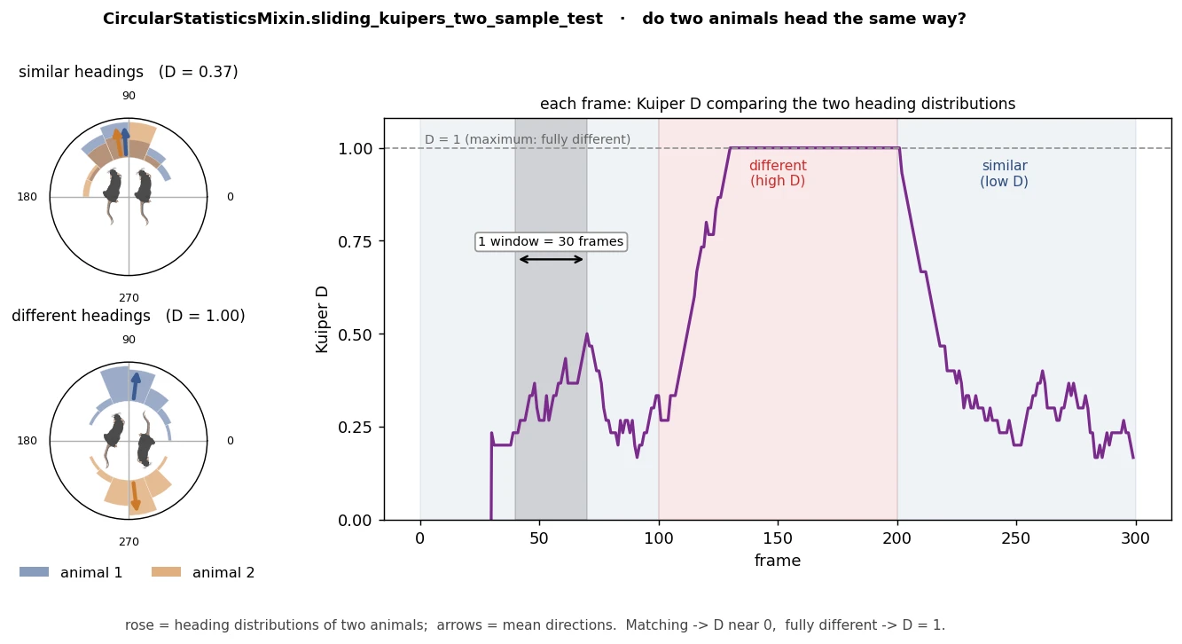
- static CircularStatisticsMixin.sliding_kuipers_two_sample_test(sample_1, sample_2, time_windows, fps)[source]
Jitted compute of Kuipers two-sample test comparing two distributions with sliding time window.
This function calculates the Kuipers two-sample test statistic for each time window, sliding through the given circular data sequences.
- Parameters
sample_1 (np.ndarray) – The first circular sample array in degrees.
sample_2 (np.ndarray) – The second circular sample array in degrees.
time_windows (np.ndarray) – An array containing the time window sizes (in seconds) for which the Kuipers two-sample test will be computed.
fps (int) – The frames per second, representing the sampling rate of the data.
- Returns
A 2D array containing the Kuipers two-sample test statistics for each time window and each time step.
- Return type
np.ndarray
- Examples
>>> data = np.random.randint(low=0, high=360, size=(100,)).astype(np.float64)
>>> D = CircularStatisticsMixin().sliding_kuipers_two_sample_test(data=data, time_windows=np.array([0.5, 5]), fps=2)
Circular correlation
- static CircularStatisticsMixin.circular_correlation(sample_1, sample_2)[source]
Jitted compute of circular correlation coefficient of two samples using the cross-correlation coefficient. Ranges from -1 to 1: 1 indicates perfect positive correlation, -1 indicates perfect negative correlation, 0 indicates no correlation.
The circular correlation coefficient is calculated as:
\[R = \frac{\sum \sin(\theta_1 - \bar{\theta}_1) \sin(\theta_2 - \bar{\theta}_2)}{\sqrt{\sum \sin^2(\theta_1 - \bar{\theta}_1) \sum \sin^2(\theta_2 - \bar{\theta}_2)}}\]Where:
\(\theta_1\) and \(\theta_2\) are the angles (in radians) from sample_1 and sample_2, respectively
\(\bar{\theta}_1\) and \(\bar{\theta}_2\) are the mean directions of sample_1 and sample_2, respectively
\(R\) is the circular correlation coefficient ranging from -1 to 1
Note
Adapted from
astropy.stats.circstats.circcorrcoef.
- Parameters
sample_1 (np.ndarray) – Angular data for e.g., Animal 1
sample_2 (np.ndarray) – Angular data for e.g., Animal 2
- Returns
The correlation between the two distributions.
- Return type
- Example
>>> sample_1 = np.array([50, 90, 20, 60, 20, 90]).astype(np.float32)
>>> sample_2 = np.array([50, 90, 70, 60, 20, 90]).astype(np.float32)
>>> CircularStatisticsMixin().circular_correlation(sample_1=sample_1, sample_2=sample_2)
>>> 0.7649115920066833
References
- 1
Mardia, K. V. (1976). Linear-circular correlation coefficients and rhythmometry. Biometrika, 63(2), 403–405.
- static CircularStatisticsMixin.sliding_circular_correlation(sample_1, sample_2, time_windows, fps)[source]
Jitted compute of correlations between two angular distributions in sliding time-windows using the cross-correlation coefficient.

Note
Values prior to the ending of the first time window will be filles with
0.\[r = \frac{\sum \sin(\theta_1 - \bar{\theta_1}) \cdot \sin(\theta_2 - \bar{\theta_2})}{\sqrt{\sum \sin^2(\theta_1 - \bar{\theta_1}) \cdot \sum \sin^2(\theta_2 - \bar{\theta_2})}}\]Where: - \(r\) is the circular correlation coefficient. - \(\theta_1\) and \(\theta_2\) are the angular data points from the two samples. - \(\bar{\theta_1}\) and \(\bar{\theta_2}\) are the mean angles of the two samples.
- Parameters
- Returns
Array of size len(sample_1) x len(time_window) with correlation coefficients.
- Return type
np.ndarray
- Example
>>> sample_1 = np.random.randint(0, 361, (200,)).astype(np.float32)
>>> sample_2 = np.random.randint(0, 361, (200,)).astype(np.float32)
>>> CircularStatisticsMixin().sliding_circular_correlation(sample_1=sample_1, sample_2=sample_2, time_windows=np.array([0.5, 1.0]), fps=10.0)
Angular hotspots & circle fitting
- static CircularStatisticsMixin.circular_hotspots(data, bins)[source]
Calculate the proportion of data points falling within circular bins.

Warning
Make sure the
binsargument do not contain overlapping bin edge definitions. E.g., bins = np.array([[270, 0], [1, 90], [91, 180], [181, 269]]) is accepted but bins = np.array([[270, 0], [0, 90], [90, 180], [180, 270]]) is not.See also
simba.data_processors.cuda.circular_statistics.sliding_circular_hotspots(),simba.mixins.circular_statistics.CircularStatisticsMixin.sliding_circular_hotspots()- Parameters
data (ndarray) – 1D array of circular data measured in degrees.
bins (ndarray) – 2D array of shape representing circular bins defining [start_degree, end_degree] inclusive.
- Returns
1D array containing the proportion of data points that fall within each specified circular bin.
- Return type
np.ndarray
- Example
>>> data = np.array([270, 360, 10, 90, 91, 180, 185, 260]).astype(np.float32)
>>> bins = np.array([[270, 90], [91, 269]])
>>> CircularStatisticsMixin().circular_hotspots(data=data, bins=bins)
>>> [0.5, 0.5]
>>> bins = np.array([[270, 0], [1, 90], [91, 180], [181, 269]])
>>> CircularStatisticsMixin().circular_hotspots(data=data, bins=bins)
>>> [0.25, 0.25, 0.25, 0.25]
- static CircularStatisticsMixin.sliding_circular_hotspots(data, bins, time_window, fps)[source]
Jitted compute of sliding circular hotspots in a dataset. Calculates circular hotspots in a time-series dataset by sliding a time window across the data and computing hotspot statistics for specified circular bins.
- Parameters
- Return np.ndarray
A 2D numpy array where each row corresponds to a time point in data, and each column represents a circular bin. The values in the array represent the proportion of data points within each bin at each time point.
Note
The function utilizes the Numba JIT compiler for improved performance.
Circular bin definitions should follow the convention where angles are specified in degrees within the range [0, 360], and the bins are defined using start and end angles inclusive. For example, (0, 90) represents the first quadrant in a circular space.
For example, bins = np.array([[270, 90], [91, 269]]) divides the space into a top and bottom circular space.
bins = np.array([[0, 179], [180, 364]]) divides the space into a left and right circular space.
Output data in the beginning of the series where a full time-window is not satisfied (e.g., first 9 observations when fps equals 10 and time_windows = [1.0], will be populated by
0.
Warning
Note that
0is noted as a bin-edge,360should not be a bin-edge. Instead, use0and359or1and360.
See also
simba.data_processors.cuda.circular_statistics.circular_hotspots(),simba.mixins.circular_statistics.CircularStatisticsMixin.sliding_circular_hotspots()- Example
>>> data = np.array([270, 360, 10, 20, 90, 91, 180, 185, 260, 265]).astype(np.float32)
>>> bins = np.array([[270, 90], [91, 269]])
>>> CircularStatisticsMixin().sliding_circular_hotspots(data=data, bins=bins, time_window=0.5, fps=10)
>>> [[-1. , -1. ],
>>>  [-1. , -1. ],
>>>  [-1. , -1. ],
>>>  [-1. , -1. ],
>>>  [ 0.5,  0. ],
>>>  [ 0.4,  0.1],
>>>  [ 0.3,  0.2],
>>>  [ 0.2,  0.3],
>>>  [ 0.1,  0.4],
>>>  [ 0. ,  0.5]]
- static CircularStatisticsMixin.fit_circle(data, max_iterations=400)[source]
Fit a circle to a dataset using the least squares method.
This function fits a circle to a dataset using the least squares method. The circle is defined by the equation:
\[X^2 + Y^2 = R^2\]Note
Adapted to numba JIT from circle-fit
hyperLSQmethod.
References
- 1
Kanatani, K., & Rangarajan, P. (2011). Hyper least squares fitting of circles and ellipses. Computational Statistics & Data Analysis, 55(6), 2197–2208.
- 2
Lapp, H. E., Salazar, M. G., & Champagne, F. A. (2023). Automated maternal behavior during early life in rodents (AMBER) pipeline. Scientific Reports, 13, 18277.
- Parameters
data (np.ndarray) – A 3D NumPy array with shape (N, M, 2). N represent frames, M represents the number of body-parts, and 2 represents x and y coordinates.
max_iterations (int) – The maximum number of iterations for fitting the circle.
- Returns
Array with shape (N, 3) with N representing frame and 3 representing (i) X-coordinate of the circle center, (ii) Y-coordinate of the circle center, and (iii) Radius of the circle
- Return type
np.ndarray
- Example
>>> data = np.array([[[5, 10], [10, 5], [15, 10], [10, 15]]])
>>> CircularStatisticsMixin().fit_circle(data=data, iter_max=88)
>>> [[10, 10, 5]]
Circular GPU methods
- simba.data_processors.cuda.circular_statistics.direction_from_three_bps(x, y, z, batch_size=15000000)[source]
Calculate the direction angle based on the coordinates of three body points using GPU acceleration.
This function computes the mean direction angle (in degrees) for a batch of coordinates provided in the form of NumPy arrays. The calculation is based on the arctangent of the difference in x and y coordinates between pairs of points. The result is a value in the range [0, 360) degrees.
See also
More CPU function, see
simba.mixins.circular_statistics.CircularStatisticsMixin.direction_three_bps()
- Parameters
x (np.ndarray) – A 2D array of shape (N, 2) containing the x-coordinates of the first body part (nose)
y (np.ndarray) – A 2D array of shape (N, 2) containing the coordinates of the second body part (left ear).
z (np.ndarray) – A 2D array of shape (N, 2) containing the coordinates of the second body part (right ear).
batch_size (Optional[int]) – The size of the batch to be processed in each iteration. Default is 15 million.
- Returns
An array of shape (N,) containing the computed direction angles in degrees.
- Return type
np.ndarray
- simba.data_processors.cuda.circular_statistics.direction_from_two_bps(x, y)[source]
Compute the directionality in degrees from two body-parts. E.g.,
napeandnose, orswim_bladderandtailwith GPU acceleration.EXPECTED RUNTIMES
FRAMES (MILLIONS)
CUDA JIT GPU (S)
2
0.0285
4
0.0404
8
0.069
16
0.1352
32
0.2711
64
0.5586
128
0.8525
256
1.6652
512
4.1223
See also
For CPU function see
simba.mixins.circular_statistics.CircularStatisticsMixin.direction_two_bps().
- Parameters
x (np.ndarray) – Size len(frames) x 2 representing x and y coordinates for first body-part.
y (np.ndarray) – Size len(frames) x 2 representing x and y coordinates for second body-part.
- Returns
Frame-wise directionality in degrees.
- Return type
np.ndarray.
- simba.data_processors.cuda.circular_statistics.instantaneous_angular_velocity(x, stride=1)[source]
Calculate the instantaneous angular velocity between angles in a given array.
This function uses CUDA to perform parallel computations on the GPU.
The angular velocity is computed using the difference in angles between the current and previous values (with a specified stride) in the array. The result is returned in degrees per unit time.
EXPECTED RUNTIMES
OBSERVATIONS/FRAMES (MILLIONS)
TIME (S)
2
0.045
4
0.098
8
0.088
16
0.227
32
0.231
64
0.514
128
0.641
256
1.43
512
2.721
1000
5.481
\[\omega = \frac{{\Delta \theta}}{{\Delta t}} = \frac{{180}}{{\pi}} \times \left( \pi - \left| \pi - \left| \theta_r - \theta_l \right| \right| \right)\]where: - \(\theta_r\) is the current angle. - \(\theta_l\) is the angle at the specified stride before the current angle. - \(\Delta t\) is the time difference between the two angles.
See also
For CPU function, see
simba.mixins.circular_statistics.CircularStatisticsMixin.instantaneous_angular_velocity()- Parameters
x (np.ndarray) – Array of angles in degrees, for which the instantaneous angular velocity will be calculated.
stride (Optional[int]) – The stride or lag (in frames) to use when calculating the difference in angles. Defaults to 1.
- Returns
Array of instantaneous angular velocities corresponding to the input angles. Velocities are in degrees per unit time.
- Return type
np.ndarray
- simba.data_processors.cuda.circular_statistics.rotational_direction(data, stride=1)[source]
Computes the rotational direction between consecutive data points in a circular space, where the angles wrap around at 360 degrees. The function uses GPU acceleration via CUDA to process the data in parallel.
The result array contains values:
0 where there is no change between points.
1 where the angle has increased in the positive direction.
2 where the angle has decreased in the negative direction.
See also
simba.mixins.circular_statistics.CircularStatisticsMixin.rotational_direction()for jitted CPU method.
- Parameters
data (np.ndarray) – 1D array of angular data (in degrees) to analyze. The data will be internally converted to radians and wrapped between [0, 360) degrees before processing.
stride (Optional[int]) – The stride or gap between data points for which the rotational direction is calculated. Default is 1.
- Returns
A 1D array of integers of the same length as data, where each element indicates the rotational direction between the current and previous point based on the stride. The first stride elements in the result will be initialized to -1 since they cannot be compared.
- Return type
np.ndarray
- Example
>>> data = np.random.randint(0, 365, (100))
>>> p = rotational_direction(data=data)
- simba.data_processors.cuda.circular_statistics.sliding_angular_diff(x, time_windows, fps)[source]
Calculate the sliding angular differences for a given time window using GPU acceleration.
This function computes the angular differences between each angle in x and the corresponding angle located at a distance determined by the time window and frame rate (fps). The results are returned as a 2D array where each row corresponds to a position in x, and each column corresponds to a different time window.
EXPECTED RUNTIMES
FRAMES
CUDA JIT GPU (S)
NUMBA CPU TIME (S)
2
0.0287
0.009
4
0.0544
0.020
8
0.1148
0.043
16
0.2204
0.086
32
0.5686
0.260
64
1.7362
0.607
128
2.5639
0.897
256
5.6997
2.454
512
29.272
12.416
See also
For CPU function, see
simba.mixins.circular_statistics.CircularStatisticsMixin.sliding_angular_diff()
\[\text{difference} = \pi - |\pi - |a_1 - a_2||\]Where: - \(a_1\) is the angle at position x. - \(a_2\) is the angle at position x - text{stride}.
- Parameters
x (np.ndarray) – 1D array of angles in degrees.
time_windows (np.ndarray) – 1D array of time windows in seconds to determine the stride (distance in frames) between angles.
fps (float) – Frame rate (frames per second) used to convert time windows to strides.
- Returns
2D array of angular differences. Each row corresponds to an angle in x, and each column corresponds to a time window.
- Return type
np.ndarray
- simba.data_processors.cuda.circular_statistics.sliding_bearing(x, stride=1, sample_rate=1)[source]
Compute the bearing between consecutive points in a 2D coordinate array using a sliding window approach using GPU acceleration.
This function calculates the angle (bearing) in degrees between each point and a point a certain number of steps ahead (defined by stride) in the 2D coordinate array x. The bearing is calculated using the arctangent of the difference in coordinates, converted from radians to degrees.
EXPECTED RUNTIMES
FRAMES / OBSERVATIONS (MILLIONS)
CUDA JIT GPU (S)
CUDA JIT GPU (STD)
2
0.0584
0.033
4
0.0981
0.04097442
8
0.0871
0.0274
16
0.2331
0.055
32
0.2213
0.0837
64
0.321
0.1053
128
0.3986
0.1917
256
0.9613
0.2957
512
2.4208
0.68659184
1000
24.83
2.1469
- Parameters
x (np.ndarray) – A 2D array of shape (n, 2) where each row represents a point with x and y coordinates. The array must be numeric.
stride (Optional[float]) – The time (multiplied by sample_rate) to look ahead when computing the bearing in seconds. Defaults to 1.
sample_rate (Optional[float]) – A multiplier applied to the stride value to determine the actual step size for calculating the bearing. E.g., frames per second. Defaults to 1. If the resulting stride is less than 1, it is automatically set to 1.
:return:A 1D array of shape (n,) containing the calculated bearings in degrees. Values outside the valid range (i.e., where the stride exceeds array bounds) are set to -1. :rtype: np.ndarray
- simba.data_processors.cuda.circular_statistics.sliding_circular_correlation_cuda(sample_1, sample_2, time_windows, fps)[source]
Compute the circular correlation coefficient between two angular signals over each sliding window (for every window length and frame), on the GPU.
Note
Angular inputs are in degrees. The result at each frame is the absolute circular cross-correlation of the window ending at that frame; incomplete windows (before the first full window) and zero-denominator windows are 0.
EXPECTED RUNTIMES
N FRAMES
MEAN (S)
SD (S)
FRAMES/S
1k
0.0010
0.0002
1.0m
10k
0.0009
0.0001
11.5m
100k
0.0020
0.0001
49.3m
1m
0.0179
0.0002
55.8m
10m
0.1698
0.0026
58.9m
100m
1.5195
0.1653
65.8m
500m
7.4178
0.6019
67.4m
NVIDIA GeForce RTX 4070
1 window=1.0s / fps=30; mean +/- SD of 3 runs; float32
angular inputs in degrees; ~112x vs CPU numba at 1m frames
See also
CPU (numba) version:
simba.mixins.circular_statistics.CircularStatisticsMixin.sliding_circular_correlation().- Parameters
sample_1 (np.ndarray) – First 1D angular signal in degrees.
sample_2 (np.ndarray) – Second 1D angular signal in degrees (same length as
sample_1).time_windows (np.ndarray) – 1D array of window lengths in seconds.
fps (float) – Frames per second (converts window lengths in seconds to frames). May be fractional (e.g. 29.97).
- Returns
2D float32 array (len(sample_1), len(time_windows)) of circular correlation per window.
- Return type
np.ndarray
- Example
>>> s1 = np.random.randint(0, 361, (200,)).astype(np.float32)
>>> s2 = np.random.randint(0, 361, (200,)).astype(np.float32)
>>> sliding_circular_correlation_cuda(sample_1=s1, sample_2=s2, time_windows=np.array([0.5, 1.0]), fps=10.0)
- simba.data_processors.cuda.circular_statistics.sliding_circular_hotspots(x, time_window, sample_rate, bins, batch_size=35000000)[source]
Calculate the proportion of data points falling within specified circular bins over a sliding time window using GPU
This function processes time series data representing angles (in degrees) and calculates the proportion of data points within specified angular bins over a sliding window. The calculations are performed in batches to accommodate large datasets efficiently.
EXPECTED RUNTIMES
FRAMES (MILLIONS)
GPU (s)
GPU (STDEV)
2
0.0219
0
4
0.0387
0.002
8
0.0809
0.015
16
0.1304
0.008
32
0.3135
0.043
64
0.593
0.054
128
1.2028
0.156
256
2.3236
0.101
512
4.9477
0.538
1024
10.266
1.351
NVIDIA GeForce RTX 4070
BATCH_SIZE: 3e+7
REPEATS 5
See also
For CPU function see
sliding_circular_hotspots().- Parameters
x (np.ndarray) – The input time series data in degrees. Should be a 1D numpy array.
time_window (float) – The size of the sliding window in seconds.
sample_rate (float) – The sample rate of the time series data (i.e., hz, fps).
bins (ndarray) – 2D array of shape representing circular bins defining [start_degree, end_degree] inclusive.
batch_size (Optional[int]) – The size of each batch for processing the data. Default is 5e+7 (50m).
- Returns
A 2D numpy array where each row corresponds to a time point in data, and each column represents a circular bin. The values in the array represent the proportion of data points within each bin at each time point. The first column represents the first bin.
- Return type
np.ndarray
- simba.data_processors.cuda.circular_statistics.sliding_circular_mean(x, time_window, sample_rate, batch_size=30000000.0)[source]
Calculate the sliding circular mean over a time window for a series of angles.
This function computes the circular mean of angles in the input array x over a specified sliding window. The circular mean is a measure of the average direction for angles, which is especially useful for angular data where traditional averaging would not be meaningful due to the circular nature of angles (e.g., 359° and 1° should average to 0°).
The calculation is performed using a sliding window approach, where the circular mean is computed for each window of angles. The function leverages GPU acceleration via CuPy for efficiency when processing large datasets.
The circular mean \(\mu\) for a set of angles is calculated using the following formula:
\[\mu = \text{atan2}\left(\frac{1}{N} \sum_{i=1}^{N} \sin(\theta_i), \frac{1}{N} \sum_{i=1}^{N} \cos(\theta_i)\right)\]\(\theta_i\) are the angles in radians within the sliding window
\(N\) is the number of samples in the window
EXPECTED RUNTIMES
FRAMES (MILLIONS)
GPU (s)
GPU (STDEV)
1
0.0755
0.07201
2
0.03908
0.00131
4
0.0726
0.00205
8
0.13196
0.00872
16
0.26056
0.01587
32
0.60962
0.07974
64
1.01012
0.02032
128
2.05793
0.15376
256
4.08802
0.14152
512
14.67234
3.66222
1000
27.43026
3.35774
See also
For CPU function see
sliding_circular_mean().- Parameters
x (np.ndarray) – Input array containing angle values in degrees. The array should be 1-dimensional.
time_window (float) – Time duration for the sliding window, in seconds. This determines the number of samples in each window based on the sample_rate.
sample_rate (int) – The number of samples per second (i.e., FPS). This is used to calculate the window size in terms of array indices.
batch_size (Optional[int]) – The maximum number of elements to process in each batch. This is used to handle large arrays by processing them in chunks to avoid memory overflow. Defaults to 3e+7 (30 million elements).
- Return np.ndarray
A 1D numpy array of the same length as x, containing the circular mean for each sliding window. Values before the window is fully populated will be set to -1.
- Example
>>> x = np.random.randint(0, 361, (i, )).astype(np.int32)
>>> results = sliding_circular_mean(x, 1, 10)
- simba.data_processors.cuda.circular_statistics.sliding_circular_range(x, time_window, sample_rate, batch_size=50000000)[source]
Computes the sliding circular range of a time series data array using GPU.
This function calculates the circular range of a time series data array using a sliding window approach. The input data is assumed to be in degrees, and the function handles the circular nature of the data by considering the circular distance between angles.
\[R = \min \left( \text{max}(\Delta \theta) - \text{min}(\Delta \theta), \, 360 - \text{max}(\Delta \theta) + \text{min}(\Delta \theta) \right)\]where:
\(\Delta \theta\) is the difference between angles within the window,
\(360\) accounts for the circular nature of the data (i.e., wrap-around at 360 degrees).
EXPECTED RUNTIMES
FRAMES (MILLIONS)
GPU (s)
GPU (STDEV)
2
0.055
0.199
4
0.115
0.005
8
0.239
0.003
16
0.398
0.023
32
0.768
0.012
64
1.596
0.04
128
3.118
0.131
256
6.84703
0.73121
512
12.36
0.122
1024
25.17
0.075
NVIDIA GeForce RTX 4070
BATCH_SIZE: 3e+7
REPEATS 5
See also
For CPU function see
sliding_circular_range().- Parameters
x (np.ndarray) – The input time series data in degrees. Should be a 1D numpy array.
time_window (float) – The size of the sliding window in seconds.
sample_rate (float) – The sample rate of the time series data (i.e., hz, fps).
batch_size (Optional[int]) – The size of each batch for processing the data. Default is 5e+7 (50m).
- Returns
A numpy array containing the sliding circular range values.
- Return type
np.ndarray
- Example
>>> x = np.random.randint(0, 361, (19, )).astype(np.int32)
>>> p = sliding_circular_range(x, 1, 10)
- simba.data_processors.cuda.circular_statistics.sliding_circular_std(x, time_window, sample_rate, batch_size=50000000)[source]
Calculate the sliding circular standard deviation of a time series data on GPU.
This function computes the circular standard deviation over a sliding window for a given time series array. The time series data is assumed to be in degrees, and the function converts it to radians for computation. The sliding window approach is used to handle large datasets efficiently, processing the data in batches.
The circular standard deviation (σ) is computed using the formula:
\[\sigma = \sqrt{-2 \cdot \log \left|\text{mean}\left(\exp(i \cdot x_{\text{batch}})\right)\right|}\]where \(x_{\text{batch}}\) is the data within the current sliding window, and \(\text{mean}\) and \(\log\) are computed in the circular (complex plane) domain.
EXPECTED RUNTIMES
FRAMES (MILLIONS)
GPU (s)
GPU (STDEV)
2
0.027
0.0009
4
0.048
0.0028
8
0.117
0.0199
16
0.163
0.0052
32
0.362
0.0571
64
0.653
0.0134
128
1.439
0.1888
256
2.836
0.1929
512
6.107
0.232
1024
22.893
5.933
NVIDIA GeForce RTX 4070
BATCH_SIZE: 3e+7
REPEATS 5
See also
For CPU function see
sliding_circular_std().- Parameters
x (np.ndarray) – The input time series data in degrees. Should be a 1D numpy array.
time_window (float) – The size of the sliding window in seconds.
sample_rate (float) – The sample rate of the time series data (i.e., hz, fps).
batch_size (Optional[int]) – The size of each batch for processing the data. Default is 5e+7 (50m).
- Returns
A numpy array containing the sliding circular standard deviation values.
- Return type
np.ndarray
- simba.data_processors.cuda.circular_statistics.sliding_kuipers_two_sample_test_cuda(sample_1, sample_2, time_windows, fps)[source]
Compute Kuiper’s two-sample test statistic between two circular signals over sliding windows, on the GPU.
Note
Each window length (
int(time_window * fps)) must be <= 512 (per-thread sort buffers). Following the CPU version, the statistic for windowsample[i-w:i]is stored at rowi, and rows before the first full window are -1. Output is (n_frames, n_time_windows) float64. Runtime grows with window length (per-thread sort).EXPECTED RUNTIMES
N FRAMES (win=30)
MEAN (S)
SD (S)
FRAMES/S
1k
0.0010
0.0002
1.0m
10k
0.0012
0.0000
8.3m
100k
0.0035
0.0002
28.4m
1m
0.0266
0.0012
37.7m
10m
0.2450
0.0065
40.8m
100m
2.3284
0.0407
42.9m
500m
12.0618
0.6098
41.5m
NVIDIA GeForce RTX 4070
window=30 frames (1.0s / 30fps); 1 time-window; mean +/- SD of 3 runs
two per-window sorts + searchsorted CDFs; runtime grows with window (max 512); ~86x vs CPU at 1m
See also
CPU (numba) version:
simba.mixins.circular_statistics.CircularStatisticsMixin.sliding_kuipers_two_sample_test().- Parameters
sample_1 (np.ndarray) – First 1D circular signal in degrees.
sample_2 (np.ndarray) – Second 1D circular signal in degrees (same length as
sample_1).time_windows (np.ndarray) – 1D array of window sizes in seconds.
fps (float) – Sampling rate of the signal (may be fractional).
- Returns
(n_frames, n_time_windows) float64 array of Kuiper’s V statistics.
- Return type
np.ndarray
- Example
>>> s1 = np.random.randint(0, 360, (5000,)).astype(np.float32)
>>> s2 = np.random.randint(0, 360, (5000,)).astype(np.float32)
>>> sliding_kuipers_two_sample_test_cuda(sample_1=s1, sample_2=s2, time_windows=np.array([0.5, 1.0]), fps=30.0)
- simba.data_processors.cuda.circular_statistics.sliding_rayleigh_z(x, time_window, sample_rate, batch_size=50000000)[source]
Computes the Rayleigh Z-statistic over a sliding window for a given time series of angles
This function calculates the Rayleigh Z-statistic, which tests the null hypothesis that the population of angles is uniformly distributed around the circle. The calculation is performed over a sliding window across the input time series, and results are computed in batches for memory efficiency.
Data is processed using GPU acceleration via CuPy, which allows for faster computation compared to a CPU-based approach.
Note
Adapted from
pingouin.circular.circ_rayleighandpycircstat.tests.rayleigh.Rayleigh Z-statistic:
The Rayleigh Z-statistic is given by:
\[R = \frac{1}{n} \sqrt{\left(\sum_{i=1}^{n} \cos(\theta_i)\right)^2 + \left(\sum_{i=1}^{n} \sin(\theta_i)\right)^2}\]where: - \(\theta_i\) are the angles in the window. - \(n\) is the number of angles in the window.
EXPECTED RUNTIMES
FRAMES (MILLIONS)
GPU (s)
GPU (STDEV)
2
0.02531
0.00328
4
0.04003
0.00533
8
0.07184
0.01016
16
0.12379
0.01608
32
0.2542
0.03084
64
0.52848
0.05978
128
1.05474
0.16997
256
1.93246
0.07944
512
4.45524
0.07773
1000
8.46498
0.33432
NVIDIA GeForce RTX 4070
BATCH_SIZE: 3e+7
REPEATS 5
See also
For CPU function see
sliding_rayleigh_z().- Parameters
x (np.ndarray) – Input array of angles in degrees. Should be a 1D numpy array.
time_window (float) – The size of the sliding window in time units (e.g., seconds).
sample_rate (float) – The sampling rate of the input time series in samples per time unit (e.g., Hz, fps).
batch_size (Optional[int]) – The number of samples to process in each batch. Default is 5e7 (50m). Reducing this value may save memory at the cost of longer computation time.
- Returns
A tuple containing two numpy arrays: - z_results: Rayleigh Z-statistics for each position in the input array where the window was fully applied. - p_results: Corresponding p-values for the Rayleigh Z-statistics.
- Return type
Tuple[np.ndarray, np.ndarray]
- simba.data_processors.cuda.circular_statistics.sliding_resultant_vector_length(x, time_window, sample_rate, batch_size=30000000.0)[source]
Calculate the sliding resultant vector length over a time window for a series of angles.
This function computes the resultant vector length (R) for each window of angles in the input array x. The resultant vector length is a measure of the concentration of angles, and it ranges from 0 to 1, where 1 indicates all angles point in the same direction, and 0 indicates uniform distribution of angles.
For a given sliding window of angles, the resultant vector length \(R\) is calculated using the following formula:
\[R = \frac{1}{N} \sqrt{\left(\sum_{i=1}^{N} \cos(\theta_i)\right)^2 + \left(\sum_{i=1}^{N} \sin(\theta_i)\right)^2}\]where:
\(\theta_i\) are the angles in radians within the sliding window
\(N\) is the number of samples in the window
The computation is performed in a sliding window manner over the entire array, utilizing GPU acceleration with CuPy for efficiency, especially on large datasets.
EXPECTED RUNTIMES
FRAMES (MILLIONS)
GPU (s)
GPU (STDEV)
2
0.04253
0.002
4
0.06979
0
8
0.14922
0.015
16
0.34029
0.062
32
0.48812
0.012
64
1.0269
0.059
128
2.16228
0.156
256
4.15671
0.027
512
11.4188
2.501
1000
28.76021
2.59123
NVIDIA GeForce RTX 4070
BATCH_SIZE: 3e+7
REPEATS 5
See also
For CPU function see
sliding_resultant_vector_length().- Parameters
x (np.ndarray) – Input array containing angle values in degrees. The array should be 1-dimensional.
time_window (float) – Time duration for the sliding window, in seconds. This determines the number of samples in each window based on the sample_rate.
sample_rate (int) – The number of samples per second (i.e., FPS). This is used to calculate the window size in terms of array indices.
batch_size (Optional[int]) – The maximum number of elements to process in each batch. This is used to handle large arrays by processing them in chunks to avoid memory overflow. Defaults to 3e+7 (30 million elements).
- Return np.ndarray
A 1D numpy array of the same length as x, containing the resultant vector length for each sliding window. Values before the window is fully populated will be set to -1.
- Example
>>> x = np.random.randint(0, 361, (5000, )).astype(np.int32)
>>> results = sliding_resultant_vector_length(x, 1, 10)