SimBA argument checks

simba.utils.checks.check_all_dfs_in_list_has_same_cols(dfs: List[DataFrame], raise_error: bool = True, source: str = '') → bool[source]

Check that all DataFrames in a list have the same column names.

This function validates that all DataFrames in the provided list contain identical column headers. It finds the intersection of all column names and identifies any missing headers that are not present in all DataFrames.

Parameters

dfs (List[pd.DataFrame]) – List of DataFrames to validate for consistent column names.
raise_error (bool) – If True, raises MissingColumnsError when column names don’t match. If False, returns False. Default: True.
source (str) – Source identifier for error messages. Default: ‘’.

Returns

True if all DataFrames have the same column names, False if they don’t match and raise_error=False.

Return type

bool

Raises

MissingColumnsError – If DataFrames have different column names and raise_error=True.

Example

>>> df1 = pd.DataFrame({'A': [1, 2], 'B': [3, 4]})
>>> df2 = pd.DataFrame({'A': [5, 6], 'B': [7, 8]})
>>> check_all_dfs_in_list_has_same_cols(dfs=[df1, df2])
True
>>> df3 = pd.DataFrame({'A': [1, 2], 'C': [3, 4]})
>>> check_all_dfs_in_list_has_same_cols(dfs=[df1, df3], raise_error=False)
False

simba.utils.checks.check_all_file_names_are_represented_in_video_log(video_info_df: DataFrame, data_paths: List[Union[str, PathLike]]) → None[source]

Helper to check that all files are represented in a dataframe of the SimBA project_folder/logs/video_info.csv file.

Parameters

video_info_df (pd.DataFrame) – List of file-paths.
data_paths (List[Union[str, os.PathLike]]) – List of file-paths.

Raises

ParametersFileError – The list is empty.

simba.utils.checks.check_ffmpeg_available(raise_error: Optional[bool] = False) → Optional[bool][source]

Helper to check of FFMpeg is available via subprocess ffmpeg.

See also

To check which encoders are available in FFMpeg installation, see simba.utils.lookups.get_ffmpeg_encoders()

Parameters: raise_error (Optional[bool]) – If True, raises FFMPEGNotFoundError if FFmpeg can’t be found. Else return False. Default False.
Returns bool: True if ffmpeg returns not None and raise_error is False. Else False.

simba.utils.checks.check_file_exist_and_readable(file_path: Union[str, PathLike], raise_error: bool = True) → bool[source]

Checks if a path points to a readable file.

Parameters

file_path (str) – Path to file on disk.

Raises

NoFilesFoundError – The file does not exist.
CorruptedFileError – The file can not be read or is zero byte size.

simba.utils.checks.check_filepaths_in_iterable_exist(file_paths: Iterable[str], name: Optional[str] = None)[source]

simba.utils.checks.check_float(name: str, value: Any, max_value: Optional[float] = None, min_value: Optional[float] = None, raise_error: bool = True, allow_zero: bool = True, allow_negative: bool = True) → Tuple[bool, str][source]

Check if variable is a valid float.

Parameters

name (str) – Name of variable
value (Any) – Value of variable
max_value (Optional[int]) – Maximum allowed value of the float. If None, then no maximum. Default: None.
Optional[int] – Minimum allowed value of the float. If None, then no minimum. Default: Non
allow_zero (Optional[bool]) – If True, do not allow float to be zero. Default: True and allow zero.
allow_negative (Optional[bool]) – If True, do not allow float to be below zero Default: True and allow negative.
raise_error (Optional[bool]) – If True, then raise error if invalid float. Default: True.

Returns

If raise_error is False, then returns size-2 tuple, with first value being a bool representing if valid float, and second value a string representing error (if valid is False, else empty string)

Return type

Tuple[bool, str]

Examples

>>> check_float(name='My_float', value=0.5, max_value=1.0, min_value=0.0)

simba.utils.checks.check_if_2d_array_has_min_unique_values(data: ndarray, min: int) → bool[source]

Check if a 2D NumPy array has at least a minimum number of unique rows.

For example, use when creating shapely Polygons or Linestrings, which typically requires at least 2 or three unique body-part coordinates.

Parameters

data (np.ndarray) – Input 2D array to be checked.
min (np.ndarray) – Minimum number of unique rows required.

Return bool

True if the input array has at least the specified minimum number of unique rows, False otherwise.

Example

>>> data = np.array([[0, 0], [0, 0], [0, 0], [0, 1]])
>>> check_if_2d_array_has_min_unique_values(data=data, min=2)
>>> True

simba.utils.checks.check_if_df_field_is_boolean(df: DataFrame, field: Union[str, List[str]], raise_error: bool = True, bool_values: Optional[Tuple[Any]] = (0, 1), df_name: Optional[str] = '')[source]

Validate that one or more DataFrame columns only contain accepted boolean labels.

Accepted values are defined by bool_values (defaults to (0, 1)), so this utility supports both numeric and custom binary encodings.

Parameters

df (pd.DataFrame) – DataFrame to validate.
field (Union[str, List[str]]) – Column name or list of column names to check.
raise_error (bool) – If True, raise CountError on invalid values. If False, return False when invalid values are detected.
bool_values (Optional[Tuple[Any]]) – Accepted values representing boolean labels.
df_name (Optional[str]) – Optional DataFrame name included in error text.

Returns

True when validation succeeds, else False if raise_error=False and invalid values are found.

Return type

bool

Raises

InvalidInputError – If field is neither str nor List[str].
CountError – If invalid values are found and raise_error=True.

Example

>>> df = pd.DataFrame({'binary_col': [0, 1, 0, 1], 'mixed_col': [0, 1, 2, 0], 'flag': [1, 0, 1, 0]})
>>> check_if_df_field_is_boolean(df=df, field='binary_col', bool_values=(0, 1))
True
>>> check_if_df_field_is_boolean(df=df, field='mixed_col', raise_error=False)
False
>>> check_if_df_field_is_boolean(df=df, field=['binary_col', 'flag'], bool_values=(0, 1))
True

simba.utils.checks.check_if_dir_exists(in_dir: Union[str, PathLike], source: Optional[str] = None, create_if_not_exist: Optional[bool] = False, raise_error: bool = True) → Union[None, bool][source]

Check if a directory path exists.

Parameters

in_dir (Union[str, os.PathLike]) – Putative directory path.
source (Optional[str]) – String source for interpretable error messaging.
create_if_not_exist (Optional[bool]) – If directory does not exist, then create it. Default False.
raise_error (Optional[bool]) – If True, raise error if dir does not exist. If False return None. Default True.

Raises

NotDirectoryError – The directory does not exist.

simba.utils.checks.check_if_filepath_list_is_empty(filepaths: List[str], error_msg: str) → None[source]

Check if a list is empty

Parameters: List[str] – List of file-paths.
Raises: NoFilesFoundError – The list is empty.

simba.utils.checks.check_if_headers_in_dfs_are_unique(dfs: List[DataFrame]) → List[str][source]

Helper to check heaaders in multiple dataframes are unique.

Parameters: dfs (List[pd.DataFrame]) – List of dataframes.
Return List[str]: List of columns headers seen in multiple dataframes. Empty if None.
Examples

>>> df_1, df_2 = pd.DataFrame([[1, 2]], columns=['My_column_1', 'My_column_2']), pd.DataFrame([[4, 2]], columns=['My_column_3', 'My_column_1'])
>>> check_if_headers_in_dfs_are_unique(dfs=[df_1, df_2])
>>> ['My_column_1']

simba.utils.checks.check_if_keys_exist_in_dict(data: dict, key: Union[str, int, tuple, List], name: Optional[str] = '', raise_error: Optional[bool] = True) → bool[source]

Check if one or more keys exist in a dictionary.

This function validates that all specified keys are present in the given dictionary. It can check for a single key or multiple keys at once.

Parameters

data (dict) – The dictionary to check for key existence.
key (Union[str, int, tuple, List]) – The key(s) to check for in the dictionary. Can be a single key or a list/tuple of keys.
name (Optional[str]) – A string identifying the source or context of the data for informative error messaging. Default: “”.
raise_error (Optional[bool]) – If True, raises InvalidInputError if any key is missing. If False, returns False instead of raising an error. Default: True.

Return bool

True if all keys exist in the dictionary, False if any key is missing (when raise_error=False).

Raises

InvalidInputError – If any of the specified keys do not exist in the dictionary and raise_error=True.

Example

>>> data = {'a': 1, 'b': 2, 'c': 3}
>>> check_if_keys_exist_in_dict(data=data, key='a')
True
>>> check_if_keys_exist_in_dict(data=data, key=['a', 'b'])
True
>>> check_if_keys_exist_in_dict(data=data, key='d', raise_error=False)
False

simba.utils.checks.check_if_list_contains_values(data: List[Union[str, int, float]], values: List[Union[str, int, float]], name: str, raise_error: bool = True) → None[source]

Helper to check if values are represeted in a list. E.g., make sure annotatations of behvaior absent and present are represented in annitation column

Parameters

data (List[Union[float, int, str]]) – List of values. E.g., annotation column represented as list.
values (List[Union[float, int, str]]) – Values to conform present. E.g., [0, 1].
name (str) – Arbitrary name of the data for more useful error msg.
raise_error (bool) – If True, raise error of not all values can be found in data. Else, print warning.

Example

>>> check_if_list_contains_values(data=[1,2, 3, 4, 0], values=[0, 1, 6], name='My_data')

simba.utils.checks.check_if_module_has_import(parsed_file: Module, import_name: str) → bool[source]

Check if a Python module has a specific import statement. For example, check if module imports argparse or circular statistics mixin.

Used for e.g., user custom feature extraction classes in simba.utils.custom_feature_extractor.CustomFeatureExtractor.

Parameters

file_path (ast.Module) – The abstract syntax tree (AST) of the Python module.
import_name (str) – The name of the module or package to check for in the import statements.
bool – True if the specified import is found in the module, False otherwise.

Example

>>> parsed_file = ast.parse(Path('/simba/misc/piotr.py').read_text())
>>> check_if_module_has_import(parsed_file=parsed_file, import_name='argparse')
>>> True

simba.utils.checks.check_if_string_value_is_valid_video_timestamp(value: str, name: str, raise_error: bool = True) → bool[source]

Helper to check if a string is in a valid HH:MM:SS format

Parameters

value (str) – Timestamp in HH:MM:SS format.
name (str) – An arbitrary string name of the timestamp.

Raises

InvalidInputError – If the timestamp is in invalid format

Example

>>> check_if_string_value_is_valid_video_timestamp(value='00:0b:10', name='My time stamp')
>>> "InvalidInputError: My time stamp is should be in the format XX:XX:XX where X is an integer between 0-9"
>>> check_if_string_value_is_valid_video_timestamp(value='00:00:10', name='My time stamp'

simba.utils.checks.check_if_valid_img(data: ndarray, source: str = '', raise_error: bool = True, greyscale: bool = False, size: Optional[Tuple[int, int]] = None, color: bool = False) → Optional[bool][source]

Check if a variable is a valid image.

Parameters

source (str) – Name of the variable and/or class origin for informative error messaging and logging.
data (np.ndarray) – Data variable to check if a valid image representation.
greyscale (bool) – Checks that the image is greyscale. Default False.
color (bool) – Checks that the image is color. Default False.
raise_error (bool) – If True, raise InvalidInputError if invalid image representation. Else, return bool.

simba.utils.checks.check_if_valid_input(name: str, input: str, options: ~typing.List[str], raise_error: bool = True) -> (<class 'bool'>, <class 'str'>)[source]

Check if string variable is valid option.

Parameters

name (str) – Atrbitrary name of variable.
input (Any) – Value of variable.
options (List[str]) – Allowed options of input
raise_error (Optional[bool]) – If True, then raise error if invalid value. Default: True.

Return bool

False if invalid. True if valid.

Return str

If invalid, then error msg. Else, empty str.

Example

>>> check_if_valid_input(name='split_eval', input='gini', options=['entropy', 'gini'])
>>> (True, '')

simba.utils.checks.check_if_valid_rgb_str(input: str, delimiter: str = ',', return_cleaned_rgb_tuple: bool = True, reverse_returned: bool = True)[source]

Helper to check if a string is a valid representation of an RGB color.

Parameters

input (str) – Value to check as string. E.g., ‘(166, 29, 12)’ or ‘22,32,999’
delimiter (str) – The delimiter between subsequent values in the rgb input string.
return_cleaned_rgb_tuple (bool) – If True, and input is a valid rgb, then returns a “clean” rgb tuple: Eg. ‘166, 29, 12’ -> (166, 29, 12). Else, returns None.
reverse_returned (bool) – If True and return_cleaned_rgb_tuple is True, reverses to returned cleaned rgb tuple (e.g., RGB becomes BGR) before returning it.

Example

>>> check_if_valid_rgb_str(input='(50, 25, 100)', return_cleaned_rgb_tuple=True, reverse_returned=True)
>>> (100, 25, 50)

simba.utils.checks.check_if_valid_rgb_tuple(data: Tuple[int, int, int], raise_error: bool = True, source: Optional[str] = None) → bool[source]

simba.utils.checks.check_if_video_corrupted(video: Union[str, PathLike, VideoCapture], frame_interval: Optional[int] = None, frame_n: Optional[int] = 20, raise_error: Optional[bool] = True) → None[source]

Check if a video file is corrupted by inspecting a set of its frames.

Note

For decent run-time regardless of video length, pass a smaller frame_n (<100).

Parameters

video_path (Union[str, os.PathLike]) – Path to the video file or cv2.VideoCapture OpenCV object.
frame_interval (Optional[int]) – Interval between frames to be checked. If None, frame_n will be used.
frame_n (Optional[int]) – Number of frames to be checked, will be sampled at large allowed interval. If None, frame_interval will be used.
raise_error (Optional[bool]) – Whether to raise an error if corruption is found. If False, prints warning.

Return None

Example

>>> check_if_video_corrupted(video_path='/Users/simon/Downloads/NOR ENCODING FExMP8.mp4')

simba.utils.checks.check_instance(source: str, instance: object, accepted_types: Union[Tuple[Any], Any], raise_error: bool = True, warning: bool = True) → bool[source]

Check if an instance is an acceptable type.

Parameters

name (str) – Arbitrary name of instance used for interpretable error msg. Can also be the name of the method.
instance (object) – A data object.
accepted_types (Union[Tuple[object], object]) – Accepted instance types. E.g., (Polygon, pd.DataFrame) or Polygon.
raise_error (Optional[bool]) – If True, raises error of instance is not of valid type, else returns bool.
warning (Optional[bool]) – If True, prints warning of instance is not of valid type, else returns bool.

simba.utils.checks.check_int(name: str, value: Any, max_value: Optional[int] = None, min_value: Optional[int] = None, unaccepted_vals: Optional[List[int]] = None, accepted_vals: Optional[List[int]] = None, allow_negative: bool = True, allow_zero: bool = True, raise_error: Optional[bool] = True) → Tuple[bool, str][source]

Check if variable is a valid integer.

Validates that a value is an integer and optionally checks it against constraints such as minimum/maximum values, accepted/unaccepted value lists, and negative/zero number restrictions.

Parameters

name (str) – Name of the variable being checked (used in error messages).
value (Any) – The value to validate as an integer.
max_value (Optional[int]) – Maximum allowed value. If None, no maximum constraint. Default None.
min_value (Optional[int]) – Minimum allowed value. If None, no minimum constraint. Default None.
unaccepted_vals (Optional[List[int]]) – List of integer values that are not accepted. If value is in this list, validation fails. Default None.
accepted_vals (Optional[List[int]]) – List of integer values that are accepted. If value is not in this list, validation fails. Default None.
allow_negative (bool) – If False, negative values will cause validation to fail. Default True.
allow_zero (bool) – If False, zero values will cause validation to fail. Default True.
raise_error (Optional[bool]) – If True, raises IntegerError when validation fails. If False, returns (False, error_message) tuple. Default True.

Returns

If raise_error is False, returns a tuple (bool, str) where bool indicates if value is valid, and str contains error message (empty string if valid). If raise_error is True and validation passes, returns (True, “”). If raise_error is True and validation fails, raises IntegerError.

Return type

Tuple[bool, str]

Raises

IntegerError – If validation fails and raise_error is True.

Example

>>> check_int(name='My_fps', value=25, min_value=1)
>>> check_int(name='Quality', value=50, min_value=0, max_value=100, raise_error=False)
>>> check_int(name='Mode', value=2, accepted_vals=[1, 2, 3])
>>> check_int(name='Count', value=-5, allow_negative=False)
>>> check_int(name='Divisor', value=0, allow_zero=False)

simba.utils.checks.check_iterable_length(source: str, val: int, exact_accepted_length: Optional[int] = None, max: Optional[int] = inf, min: int = 1, raise_error: bool = True) → bool[source]

simba.utils.checks.check_minimum_roll_windows(roll_windows_values: List[int], minimum_fps: float) → List[int][source]

Remove any rolling temporal window that are shorter than a single frame in any of the videos within the project.

Parameters

roll_windows_values (List[int]) – Rolling temporal windows represented as frame counts. E.g., [10, 15, 30, 60]
minimum_fps (float) – The lowest fps of the videos that are to be analyzed. E.g., 10.

Return List[int]

roll_windows_values without impassable windows.

simba.utils.checks.check_nvidea_gpu_available(raise_error: bool = False) → bool[source]: Helper to check of NVIDEA GPU is available via nvidia-smi. returns bool: True if nvidia-smi returns not None. Else False.

simba.utils.checks.check_same_files_exist_in_all_directories(dirs: List[Union[str, PathLike]], raise_error: bool = False, file_type: str = 'csv') → bool[source]

Check if the same files of a given type exist in all specified directories.

Parameters

dirs (List[Union[str, os.PathLike]]) – List of directory paths to check.
raise_error (bool) – If True, raises an error when file names do not match across directories. Defaults to False.
raise_error – File extension (without the dot) to check for (e.g., ‘csv’, ‘txt’). Defaults to ‘csv’.

simba.utils.checks.check_same_number_of_rows_in_dfs(dfs: List[DataFrame]) → bool[source]

Helper to check that each dataframe in list contains an equal number of rows

Parameters: dfs (List[pd.DataFrame]) – List of dataframes.
Return bool: True if dataframes has an equal number of rows. Else False.

>>> df_1, df_2 = pd.DataFrame([[1, 2], [1, 2]]), pd.DataFrame([[4, 2], [9, 3], [1, 5]])
>>> check_same_number_of_rows_in_dfs(dfs=[df_1, df_2])
>>> False
>>> df_1, df_2 = pd.DataFrame([[1, 2], [1, 2]]), pd.DataFrame([[4, 2], [9, 3]])
>>> True

simba.utils.checks.check_str(name: str, value: Any, options: Optional[Union[Tuple[Any], List[Any], Iterable[Any]]] = (), allow_blank: bool = False, invalid_options: Optional[Union[List[str], Tuple[str]]] = None, raise_error: bool = True, invalid_substrs: Optional[Union[List[str], Tuple[str]]] = None) → Tuple[bool, str][source]

Check if variable is a valid string.

Parameters

name (str) – Name of variable
value (Any) – Value of variable
options (Optional[Tuple[Any]]) – Tuple of allowed strings. If empty tuple, then any string allowed. Default: ().
allow_blank (Optional[bool]) – If True, allow empty string. Default: False.
raise_error (Optional[bool]) – If True, then raise error if invalid string. Default: True.
invalid_options (Optional[List[str]]) – If not None, then a list of strings that are invalid.
invalid_substrs (Optional[List[str]]) – If not None, then a list of characters or substrings that are not allowed in the string.

Returns

If raise_error is False, then returns size-2 Tuple, with first value being a bool representing if valid string, and second value a string representing error reason (if valid is False, else empty string).

Return type

Tuple[bool, str]

Examples

>>> check_str(name='split_eval', input='gini', options=['entropy', 'gini'])

simba.utils.checks.check_that_column_exist(df: DataFrame, column_name: Union[str, PathLike, List[str]], file_name: str, raise_error: bool = True) → Union[None, bool][source]

Check if single named field or a list of fields exist within a dataframe.

Parameters

df (pd.DataFrame) – The DataFrame to check for column existence.
column_name (Union[str, os.PathLike, List[str]]) – Name or names of field(s) to check for existence.
file_name (str) – Path of df on disk (used for error messages).
raise_error (bool) – If True, raises ColumnNotFoundError if column doesn’t exist. If False, returns bool. Default: True.

Returns

True if all columns exist, False if any column is missing (when raise_error=False), None if raise_error=True and all columns exist.

Return type

Union[None, bool]

Raises

ColumnNotFoundError – The column_name does not exist within df.

Example

>>> df = pd.DataFrame({'A': [1, 2], 'B': [3, 4]})
>>> check_that_column_exist(df=df, column_name='A', file_name='test.csv')
True
>>> check_that_column_exist(df=df, column_name=['A', 'B'], file_name='test.csv')
True
>>> check_that_column_exist(df=df, column_name='C', file_name='test.csv', raise_error=False)
False

simba.utils.checks.check_that_dir_has_list_of_filenames(dir: Union[str, PathLike], file_name_lst: List[str], file_type: Optional[str] = 'csv')[source]

Check that all file names in a list has an equivalent file in a specified directory. E.g., check if all files in the outlier corrected folder has an equivalent file in the featurues_extracted directory.

Example

>>> file_name_lst = glob.glob('/Users/simon/Desktop/envs/troubleshooting/two_black_animals_14bp/project_folder/csv/outlier_corrected_movement' + '/*.csv')
>>> check_that_dir_has_list_of_filenames(dir = '/Users/simon/Desktop/envs/troubleshooting/two_black_animals_14bp/project_folder/csv/features_extracted', file_name_lst=file_name_lst)

simba.utils.checks.check_that_directory_is_empty(directory: Union[str, PathLike], raise_error: Optional[bool] = True) → None[source]

Checks if a directory is empty. If the directory has content, then returns False or raises DirectoryNotEmptyError.

Parameters: directory (str) – Directory to check.
Raises: DirectoryNotEmptyError – If directory contains files.

simba.utils.checks.check_that_hhmmss_start_is_before_end(start_time: str, end_time: str, name: str, raise_error: bool = True) → bool[source]

Helper to check that a start time in HH:MM:SS or HH:MM:SS:MS format is before an end time in HH:MM:SS or HH:MM:SS:MS format

Parameters

start_time (str) – Period start time in HH:MM:SS format.
end_time (str) – Period end time in HH:MM:SS format.
name (int) – Name of the variable

Raises

InvalidInputError – If end time is before the start time.

Example

>>> check_that_hhmmss_start_is_before_end(start_time='00:00:05', end_time='00:00:01', name='My time period')
>>> "InvalidInputError: My time period has an end-time which is before the start-time"
>>> check_that_hhmmss_start_is_before_end(start_time='00:00:01', end_time='00:00:05')

simba.utils.checks.check_umap_hyperparameters(hyper_parameters: Dict[str, Any]) → None[source]

Checks if dictionary of paramameters (umap, scaling, etc) are valid for grid-search umap dimensionality reduction .

Parameters: hyper_parameters (dict) – Dictionary holding umap hyerparameters.
Raises: InvalidInputError – If any input is invalid
Example

>>> check_umap_hyperparameters(hyper_parameters={'n_neighbors': [2], 'min_distance': [0.1], 'spread': [1], 'scaler': 'MIN-MAX', 'variance': 0.2})

simba.utils.checks.check_valid_array(data: ndarray, source: Optional[str] = '', accepted_ndims: Optional[Union[Tuple[int], Any]] = None, accepted_sizes: Optional[List[int]] = None, accepted_axis_0_shape: Optional[Union[List[int], Tuple[int]]] = None, accepted_axis_1_shape: Optional[Union[List[int], Tuple[int]]] = None, accepted_dtypes: Optional[Union[List[Union[str, Type]], Tuple[Union[str, Type]], Iterable[Any]]] = None, accepted_values: Optional[List[Any]] = None, accepted_shapes: Optional[List[Tuple[int]]] = None, min_axis_0: Optional[int] = None, max_axis_1: Optional[int] = None, min_axis_1: Optional[int] = None, min_value: Optional[Union[float, int]] = None, max_value: Optional[Union[float, int]] = None, raise_error: bool = True) → Union[None, bool][source]

Check if the given array satisfies specified criteria regarding its dimensions, shape, and data type.

Parameters

data (np.ndarray) – The numpy array to be checked.
source (Optional[str]) – A string identifying the source, name, or purpose of the array for interpretable error messaging.
accepted_ndims (Optional[Union[Tuple[int], Any]]) – List of tuples representing acceptable dimensions. If provided, checks whether the array’s number of dimensions matches any tuple in the list.
accepted_sizes (Optional[List[int]]) – List of acceptable sizes for the array’s shape. If provided, checks whether the length of the array’s shape matches any value in the list.
accepted_axis_0_shape (Optional[Union[List[int], Tuple[int]]]) – List of accepted number of rows of 2-dimensional array. Will also raise error if value passed and input is not a 2-dimensional array.
accepted_axis_1_shape (Optional[Union[List[int], Tuple[int]]]) – List of accepted number of columns or fields of 2-dimensional array. Will also raise error if value passed and input is not a 2-dimensional array.
accepted_dtypes (Optional[Union[List[Union[str, Type]], Tuple[Union[str, Type]], Iterable[Any]]]) – List of acceptable data types for the array. If provided, checks whether the array’s data type matches any string in the list.
accepted_values (Optional[List[Any]]) – List of acceptable values that can be present in the array.
accepted_shapes (Optional[List[Tuple[int]]]) – List of acceptable shapes for the array. If provided, checks whether the array’s shape matches any tuple in the list.
min_axis_0 (Optional[int]) – Minimum number of rows required for the array.
max_axis_1 (Optional[int]) – Maximum number of columns allowed for the array.
min_axis_1 (Optional[int]) – Minimum number of columns required for the array.
min_value (Optional[Union[float, int]]) – Minimum value allowed in the array.
max_value (Optional[Union[float, int]]) – Maximum value allowed in the array.
raise_error (bool) – If True, raises ArrayError if validation fails. If False, returns bool. Default: True.

Returns

True if array passes all validation checks, False if validation fails (when raise_error=False), None if raise_error=True and validation passes.

Return type

Union[None, bool]

Example

>>> data = np.array([[1, 2], [3, 4]])
>>> check_valid_array(data, source="Example", accepted_ndims=(2,), accepted_sizes=[2], accepted_dtypes=[np.int64])
True
>>> check_valid_array(data, source="Example", min_axis_0=3, raise_error=False)
False

simba.utils.checks.check_valid_boolean(value: Union[Any, List[Any]], source: Optional[str] = '', raise_error: Optional[bool] = True)[source]

Check if a value or list of values contains only valid boolean values.

This function validates that the input value(s) are valid Python boolean values (True or False). It can handle single values or lists of values, and provides flexible error handling options.

Parameters

value (Union[Any, List[Any]]) – Single value or list of values to validate for boolean type.
source (Optional[str]) – Source identifier for error messages. Default: ‘’.
raise_error (Optional[bool]) – If True, raises InvalidInputError when non-boolean values are found. If False, returns False. Default: True.

Returns

True if all values are valid booleans, False if any non-boolean values found and raise_error=False.

Return type

bool

Raises

InvalidInputError – If non-boolean values are found and raise_error=True.

Example

>>> check_valid_boolean(True)
True
>>> check_valid_boolean([True, False, True])
True
>>> check_valid_boolean([True, 1, False], raise_error=False)
False
>>> check_valid_boolean('not_bool', raise_error=False)
False

simba.utils.checks.check_valid_codec(codec: str, raise_error: bool = True, source: str = '')[source]

Validate that a codec string is available in the current FFmpeg installation.

Checks if the provided codec name exists in the list of available FFmpeg encoders by querying FFmpeg directly. This ensures the codec can be used for video encoding/decoding.

Note

This function requires FFmpeg to be installed and available in the system PATH. The function queries FFmpeg for available encoders at runtime, so it will reflect the actual encoders available in your FFmpeg installation.

See also

To get a list of all available encoders, see get_ffmpeg_encoders(). To check if FFmpeg is available, see check_ffmpeg_available().

Parameters

codec (str) – The codec name to validate (e.g., ‘libx264’, ‘h264_nvenc’, ‘libvpx-vp9’).
raise_error (bool) – If True, raises InvalidInputError when codec is invalid. If False, returns False. Default: True.
source (str) – Source identifier for error messages. Used when raising exceptions. Default: ‘’.

Returns

True if codec is valid, False if invalid and raise_error=False.

Return type

bool

Raises

InvalidInputError – If codec is not valid and raise_error=True.

Example

>>> check_valid_codec(codec='libx264')
>>> check_valid_codec(codec='h264_nvenc', source='my_function')
>>> is_valid = check_valid_codec(codec='invalid_codec', raise_error=False)

simba.utils.checks.check_valid_cpu_pool(value: Any, source: str = '', max_cores: Optional[int] = None, min_cores: Optional[int] = None, accepted_cores: Optional[Union[List[int], Tuple[int, ...], int]] = None, raise_error: bool = True) → bool[source]

Validates that a value is a valid multiprocessing.Pool instance and optionally checks core count constraints.

Parameters

value (Any) – The value to validate. Must be an instance of multiprocessing.pool.Pool.
source (str) – Optional source identifier for error messages. Default is empty string.
max_cores (Optional[int]) – Optional maximum number of processes allowed in the pool. If provided, validates that pool._processes <= max_cores.
min_cores (Optional[int]) – Optional minimum number of processes required in the pool. If provided, validates that pool._processes >= min_cores.
accepted_cores (Optional[Union[List[int], Tuple[int, ...], int]]) – Optional exact or list of acceptable process counts. If an int, validates that pool._processes == accepted_cores. If a list/tuple of ints, validates that pool._processes is in accepted_cores. All values must be positive integers.
raise_error (bool) – If True, raises InvalidInputError on validation failure. If False, returns False on failure. Default is True.

Return bool

True if validation passes, False if validation fails and raise_error is False.

Raises

InvalidInputError – If value is not a valid Pool instance, if core count constraints are violated, if accepted_cores contains invalid types, or if raise_error is True.

Example

>>> import multiprocessing
>>> pool = multiprocessing.Pool(processes=4)
>>> check_valid_cpu_pool(value=pool, source='test', max_cores=8, min_cores=2)
>>> True
>>> check_valid_cpu_pool(value=pool, source='test', accepted_cores=[4, 8, 16])
>>> True
>>> check_valid_cpu_pool(value=pool, source='test', accepted_cores=4)
>>> True

simba.utils.checks.check_valid_dataframe(df: DataFrame, source: Optional[str] = '', valid_dtypes: Optional[Tuple[Any]] = None, required_fields: Optional[List[str]] = None, min_axis_0: Optional[int] = None, min_axis_1: Optional[int] = None, max_axis_0: Optional[int] = None, max_axis_1: Optional[int] = None, allow_duplicate_col_names=True, accepted_rows: Optional[Union[int, Tuple[int]]] = None)[source]

Validate a DataFrame against various criteria.

This function performs comprehensive validation of a pandas DataFrame including data types, dimensions, required columns, and duplicate column names. It raises exceptions for any validation failures.

Parameters

df (pd.DataFrame) – The DataFrame to validate.
source (Optional[str]) – Source identifier for error messages. Default: “”.
valid_dtypes (Optional[Tuple[Any]]) – Tuple of allowed data types. If None, no dtype validation. Default: None.
required_fields (Optional[List[str]]) – List of required column names. If None, no field validation. Default: None.
min_axis_0 (Optional[int]) – Minimum number of rows required. If None, no minimum row validation. Default: None.
min_axis_1 (Optional[int]) – Minimum number of columns required. If None, no minimum column validation. Default: None.
max_axis_0 (Optional[int]) – Maximum number of rows allowed. If None, no maximum row validation. Default: None.
max_axis_1 (Optional[int]) – Maximum number of columns allowed. If None, no maximum column validation. Default: None.
allow_duplicate_col_names (bool) – If False, raises error for duplicate column names. Default: True.

Returns

None if validation passes.

Return type

None

Raises

InvalidInputError – If any validation criteria are not met.

Example

>>> df = pd.DataFrame({'A': [1, 2], 'B': [3, 4]})
>>> check_valid_dataframe(df=df, required_fields=['A', 'B'], min_axis_0=1)
>>> check_valid_dataframe(df=df, valid_dtypes=(int,), max_axis_1=2)
>>> check_valid_dataframe(df=df, allow_duplicate_col_names=False)

simba.utils.checks.check_valid_device(device: Union[typing_extensions.Literal['cpu'], int], raise_error: bool = True) → bool[source]

Validate a compute device specification, ensuring it is either ‘cpu’ or a valid GPU index.

This function validates that a device specification is valid for use with PyTorch/CUDA operations. It checks if the device is either ‘cpu’ for CPU usage or a valid integer representing a CUDA device index.

Parameters

device (Union[Literal['cpu'], int]) – The device to validate. Should be the string ‘cpu’ for CPU usage, or an integer representing a CUDA device index (e.g., 0 for ‘cuda:0’).
raise_error (bool) – If True, raises InvalidInputError or SimBAGPUError when the device is invalid. If False, returns False instead of raising errors. Default: True.

Returns

True if the device is valid, False if it’s invalid and raise_error=False.

Return type

bool

Raises

InvalidInputError – If the device format is invalid and raise_error=True.
SimBAGPUError – If the GPU device is not available or not valid and raise_error=True.

Example

>>> check_valid_device('cpu')
True
>>> check_valid_device(0)  # GPU 0
True
>>> check_valid_device(5, raise_error=False)  # Non-existent GPU
False
>>> check_valid_device('gpu', raise_error=False)  # Invalid format
False

simba.utils.checks.check_valid_dict(x: dict, valid_key_dtypes: Optional[Tuple[Any]] = None, valid_values_dtypes: Optional[Tuple[Any, ...]] = None, valid_keys: Optional[Union[Tuple[Any], List[Any]]] = None, max_len_keys: Optional[int] = None, min_len_keys: Optional[int] = None, required_keys: Optional[Tuple[Any, ...]] = None, max_value: Optional[Union[float, int]] = None, min_value: Optional[Union[float, int]] = None, source: Optional[str] = None)[source]

Validate a dictionary against various criteria.

This function performs comprehensive validation of a dictionary including key/value data types, key constraints, required keys, and numeric value ranges. It raises exceptions for any validation failures.

Parameters

x (dict) – The dictionary to validate.
valid_key_dtypes (Optional[Tuple[Any]]) – Tuple of allowed data types for dictionary keys. If None, no key type validation. Default: None.
valid_values_dtypes (Optional[Tuple[Any, ...]]) – Tuple of allowed data types for dictionary values. If None, no value type validation. Default: None.
valid_keys (Optional[Union[Tuple[Any], List[Any]]]) – Tuple or list of valid key names. If None, no key name validation. Default: None.
max_len_keys (Optional[int]) – Maximum number of keys allowed. If None, no maximum key count validation. Default: None.
min_len_keys (Optional[int]) – Minimum number of keys required. If None, no minimum key count validation. Default: None.
required_keys (Optional[Tuple[Any, ...]]) – Tuple of required key names. If None, no required key validation. Default: None.
max_value (Optional[Union[float, int]]) – Maximum numeric value allowed for numeric values. If None, no maximum value validation. Default: None.
min_value (Optional[Union[float, int]]) – Minimum numeric value allowed for numeric values. If None, no minimum value validation. Default: None.
source (Optional[str]) – Source identifier for error messages. If None, uses function name. Default: None.

Returns

None if validation passes.

Return type

None

Raises

InvalidInputError – If any validation criteria are not met.

Example

>>> check_valid_dict(x={'a': 1, 'b': 2}, valid_key_dtypes=(str,), valid_values_dtypes=(int,))
>>> check_valid_dict(x={'key1': 10, 'key2': 20}, required_keys=('key1',), min_value=5, max_value=25)
>>> check_valid_dict(x={'x': 1, 'y': 2}, valid_keys=('x', 'y', 'z'), min_len_keys=2)

simba.utils.checks.check_valid_extension(path: Union[str, PathLike], accepted_extensions: Union[List[str], str])[source]

Checks if the file extension of the provided path is in the list of accepted extensions.

Parameters

file_path (Union[str, os.PathLike]) – The path to the file whose extension needs to be checked.
accepted_extensions (List[str]) – A list of accepted file extensions. E.g., [‘pickle’, ‘csv’].

simba.utils.checks.check_valid_hex_color(color_hex: str, raise_error: Optional[bool] = True) → bool[source]

Check if given string represents a valid hexadecimal color code.

Parameters

color_hex (str) – A string representing a hexadecimal color code, either in the format ‘#RRGGBB’ or ‘#RGB’.
raise_error (bool) – If True, raise an exception when the color_hex is invalid; if False, return False instead. Default is True.

Return bool

True if the color_hex is a valid hexadecimal color code; False otherwise (if raise_error is False).

Raises

IntegerError – If the color_hex is an invalid hexadecimal color code and raise_error is True.

simba.utils.checks.check_valid_img_path(path: Union[str, PathLike], raise_error: bool = True)[source]

Check if a file path is a valid image file.

This function validates that a file path exists, is readable, and can be opened as an image file using OpenCV. It performs basic image file validation by attempting to read the file with cv2.imread.

Parameters

path (Union[str, os.PathLike]) – Path to the image file to validate.
raise_error (bool) – If True, raises InvalidInputError when file is not a valid image. If False, returns False. Default: True.

Returns

True if the file is a valid image file, False if it’s not valid and raise_error=False.

Return type

bool

Raises

InvalidInputError – If the file is not a valid image file and raise_error=True.

Example

>>> check_valid_img_path('/path/to/image.jpg')
True
>>> check_valid_img_path('/path/to/invalid.txt', raise_error=False)
False
>>> check_valid_img_path('/path/to/corrupted.png', raise_error=False)
False

simba.utils.checks.check_valid_lst(data: list, source: Optional[str] = '', valid_dtypes: Optional[Union[Tuple[Any], List[Any], Any]] = None, valid_values: Optional[List[Any]] = None, min_len: Optional[int] = 1, max_len: Optional[int] = None, min_value: Optional[float] = None, exact_len: Optional[int] = None, raise_error: Optional[bool] = True) → bool[source]

Check the validity of a list based on passed criteria.

Parameters

data (list) – The input list to be validated.
source (Optional[str]) – A string indicating the source or context of the data for informative error messaging.
valid_dtypes (Optional[Union[Tuple[Any], List[Any], Any]]) – A tuple, list, or single type of accepted data types. If provided, check if all elements in the list have data types in this collection.
valid_values (Optional[List[Any]]) – A list of accepted list values. If provided, check if all elements in the list have matching values in this list.
min_len (Optional[int]) – The minimum allowed length of the list. Default: 1.
max_len (Optional[int]) – The maximum allowed length of the list.
min_value (Optional[float]) – The minimum value allowed for numeric elements in the list.
exact_len (Optional[int]) – The exact length required for the list. If provided, overrides min_len and max_len.
raise_error (Optional[bool]) – If True, raise an InvalidInputError if any validation fails. If False, return False instead of raising an error. Default: True.

Return bool

True if all validation criteria are met, False otherwise.

Example

>>> check_valid_lst(data=[1, 2, 'three'], valid_dtypes=(int, str), min_len=2, max_len=5)
True
>>> check_valid_lst(data=[1, 2, 3], valid_dtypes=(int,), exact_len=3)
True
>>> check_valid_lst(data=[1, 2, 3], min_value=0, raise_error=False)
True

simba.utils.checks.check_valid_polygon(polygon: Union[ndarray, Polygon], raise_error: bool = True, name: Optional[str] = None) → Optional[bool][source]

Validates whether the given polygon is a valid geometric shape.

Parameters

polygon (Union[np.ndarray, Polygon]) – The polygon to validate, either as a NumPy array of shape (N, 2) or a shapely Polygon object.
raise_error (bool) – If True, raises an InvalidInputError if the polygon is invalid; otherwise, returns False.
name (Optional[str]) – An optional name for the polygon to include in error messages.

Returns

True if the polygon is valid, False if invalid (and raise_error is False), or None if an error is raised.

simba.utils.checks.check_valid_tuple(x: tuple, source: Optional[str] = '', accepted_lengths: Optional[Tuple[int]] = None, valid_dtypes: Optional[Tuple[Any]] = None, minimum_length: Optional[int] = None, accepted_values: Optional[Iterable[Any]] = None, min_integer: Optional[int] = None, raise_error: bool = True) → bool[source]

Validate a tuple against various criteria.

This function performs comprehensive validation of a tuple including length constraints, data types, minimum values, and accepted values. It raises exceptions for any validation failures.

Parameters

x (tuple) – The tuple to validate.
source (Optional[str]) – Source identifier for error messages. Default: “”.
accepted_lengths (Optional[Tuple[int]]) – Tuple of accepted lengths. If None, no length validation. Default: None.
valid_dtypes (Optional[Tuple[Any]]) – Tuple of allowed data types for tuple elements. If None, no dtype validation. Default: None.
minimum_length (Optional[int]) – Minimum length required. If None, no minimum length validation. Default: None.
accepted_values (Optional[Iterable[Any]]) – Iterable of accepted values for tuple elements. If None, no value validation. Default: None.
min_integer (Optional[int]) – Minimum value for integer elements. If None, no integer validation. Default: None.

Returns

None if validation passes.

Return type

None

Raises

InvalidInputError – If any validation criteria are not met.

Example

>>> check_valid_tuple(x=(1, 2, 3), accepted_lengths=(2, 3), valid_dtypes=(int,))
>>> check_valid_tuple(x=('a', 'b'), minimum_length=2, accepted_values=['a', 'b', 'c'])
>>> check_valid_tuple(x=(5, 10, 15), min_integer=5)

simba.utils.checks.check_valid_url(url: str, raise_error: bool = False, source: str = '') → bool[source]

Check if a string is a valid URL (http, https, or ftp).

Parameters

url (str) – The string to validate as a URL.
raise_error (bool) – If True, raises InvalidInputError when the URL is invalid. Default: False.
source (str) – Source identifier for error messages when raise_error=True. Default: ‘’.

Returns

True if the string is a valid URL, False otherwise.

simba.utils.checks.check_video_and_data_frm_count_align(video: Union[str, PathLike, VideoCapture], data: Union[str, PathLike, DataFrame], name: Optional[str] = '', raise_error: Optional[bool] = True) → Union[None, bool][source]

Check if the frame count of a video matches the row count of a data file.

Parameters

video (Union[str, os.PathLike, cv2.VideoCapture]) – Path to the video file or cv2.VideoCapture object.
data (Union[str, os.PathLike, pd.DataFrame]) – Path to the data file or DataFrame containing the data.
name (Optional[str]) – Name of the video (optional for interpretable error msgs).
raise_error (Optional[bool]) – Whether to raise an error if the counts don’t align (default is True). If False, prints warning.

Return None

Example

>>> data_1 = '/Users/simon/Desktop/envs/simba/troubleshooting/mouse_open_field/project_folder/csv/outlier_corrected_movement_location/SI_DAY3_308_CD1_PRESENT.csv'
>>> video_1 = '/Users/simon/Desktop/envs/simba/troubleshooting/mouse_open_field/project_folder/frames/output/ROI_analysis/SI_DAY3_308_CD1_PRESENT.mp4'
>>> check_video_and_data_frm_count_align(video=video_1, data=data_1, raise_error=True)

simba.utils.checks.check_video_has_rois(roi_dict: Dict[str, DataFrame], roi_names: Optional[List[str]] = None, video_names: Optional[List[str]] = None, source: str = 'roi dict', raise_error: bool = True)[source]

Check that specified videos all have user-defined ROIs with specified names.

This function validates that all specified videos contain the required ROIs (Regions of Interest) with the specified names. It checks across all ROI types: rectangles, circles, and polygons.

Note

To get roi dictionary, see simba.mixins.config_reader.ConfigReader.read_roi_data().

Parameters

roi_dict (Dict[str, pd.DataFrame]) – Dictionary containing ROI dataframes with keys for rectangles, circles, and polygons.
roi_names (Optional[List[str]]) – List of ROI names to check for. If None, uses all unique ROI names from the data. Default: None.
video_names (Optional[List[str]]) – List of video names to check. If None, uses all unique video names from the data. Default: None.
source (str) – A string identifying the source or context for informative error messaging. Default: ‘roi dict’.
raise_error (bool) – If True, raises NoROIDataError if any videos are missing required ROIs. If False, returns tuple with validation result and missing ROIs. Default: True.

Returns

If raise_error=True: None if all validations pass, raises exception if validation fails. If raise_error=False: Tuple of (bool, dict) where bool indicates success and dict contains missing ROIs by video.

Return type

Union[None, Tuple[bool, Dict[str, List[str]]]]

Raises

NoROIDataError – If any videos are missing required ROIs and raise_error=True.

Example

>>> roi_dict = {
...     'rectangles': pd.DataFrame({'Video': ['video1'], 'Name': ['ROI1']}),
...     'circles': pd.DataFrame({'Video': ['video1'], 'Name': ['ROI2']}),
...     'polygons': pd.DataFrame({'Video': ['video1'], 'Name': ['ROI3']})
... }
>>> check_video_has_rois(roi_dict=roi_dict, roi_names=['ROI1', 'ROI2'], video_names=['video1'])
True
>>> check_video_has_rois(roi_dict=roi_dict, roi_names=['ROI1', 'ROI4'], video_names=['video1'], raise_error=False)
(False, {'video1': ['ROI4']})

simba.utils.checks.get_fn_ext(filepath: ~typing.Union[~os.PathLike, str]) -> (<class 'str'>, <class 'str'>, <class 'str'>)[source]

Split file path into three components: (i) directory, (ii) file name, and (iii) file extension.

Parameters: filepath (str) – Path to file.
Return str: File directory name
Return str: File name
Return str: File extension
Example

>>> get_fn_ext(filepath='C:/My_videos/MyVideo.mp4')
>>> ('My_videos', 'MyVideo', '.mp4')

simba.utils.checks.is_img_bw(img: ndarray, raise_error: bool = True, source: Optional[str] = '') → bool[source]

Check if an image is binary black and white.

This function validates that an image contains only two pixel values: 0 (black) and 255 (white). It checks all unique pixel values in the image and ensures they are exactly these two values.

Parameters

img (np.ndarray) – The image array to validate for binary black and white format.
raise_error (bool) – If True, raises InvalidInputError when image is not binary black and white. If False, returns False. Default: True.
source (Optional[str]) – Source identifier for error messages. Default: ‘’.

Returns

True if the image is binary black and white, False if it’s not and raise_error=False.

Return type

bool

Raises

InvalidInputError – If the image is not binary black and white and raise_error=True.

Example

>>> bw_img = np.array([[0, 255], [255, 0]], dtype=np.uint8)
>>> is_img_bw(bw_img)
True
>>> gray_img = np.array([[128, 200], [50, 100]], dtype=np.uint8)
>>> is_img_bw(gray_img, raise_error=False)
False

simba.utils.checks.is_img_greyscale(img: ndarray, raise_error: bool = True, source: Optional[str] = '') → bool[source]

Check if an image is greyscale.

This function validates that an image is in greyscale format by checking that it has exactly 2 dimensions (height and width). Greyscale images have a single channel and are represented as 2D arrays.

Parameters

img (np.ndarray) – The image array to validate for greyscale format.
raise_error (bool) – If True, raises InvalidInputError when image is not greyscale. If False, returns False. Default: True.
source (Optional[str]) – Source identifier for error messages. Default: ‘’.

Returns

True if the image is greyscale, False if it’s not and raise_error=False.

Return type

bool

Raises

InvalidInputError – If the image is not greyscale and raise_error=True.

Example

>>> gray_img = np.array([[128, 200], [50, 100]], dtype=np.uint8)
>>> is_img_greyscale(gray_img)
True
>>> color_img = np.array([[[128, 200, 50], [100, 150, 75]]], dtype=np.uint8)
>>> is_img_greyscale(color_img, raise_error=False)
False

simba.utils.checks.is_lxc_container() → bool[source]

Helper to check if the current environment is inside a LXC Linux container.

Note

See GitHub issue 457 for origin - https://github.com/sgoldenlab/simba/issues/457#issuecomment-3052631284 Thanks Heinrich2818 - https://github.com/Heinrich2818

Returns: True if current environment is a LXC linux container, False if not.
Return type: bool

simba.utils.checks.is_valid_video_file(file_path: Union[str, PathLike], raise_error: bool = True)[source]

Check if a file path is a valid video file.

This function validates that a file path exists, is readable, and can be opened as a video file using OpenCV. It performs basic video file validation by attempting to open the file with cv2.VideoCapture.

Parameters

file_path (Union[str, os.PathLike]) – Path to the video file to validate.
raise_error (bool) – If True, raises InvalidFilepathError when file is not a valid video. If False, returns False. Default: True.

Returns

True if the file is a valid video file, False if it’s not valid and raise_error=False.

Return type

bool

Raises

InvalidFilepathError – If the file is not a valid video file and raise_error=True.

Example

>>> is_valid_video_file('/path/to/video.mp4')
True
>>> is_valid_video_file('/path/to/invalid.txt', raise_error=False)
False
>>> is_valid_video_file('/path/to/corrupted.mp4', raise_error=False)
False

simba.utils.checks.is_video_color(video: Union[str, PathLike, VideoCapture]) → bool[source]

Determines whether a video is in color or greyscale.

Parameters: video (Union[str, os.PathLike, cv2.VideoCapture]) – The video source, either a cv2.VideoCapture object or a path to a file on disk.
Returns: Returns True if the video is in color (has more than one channel), and False if the video is greyscale (single channel).
Return type: bool

simba.utils.checks.is_windows_path(value)[source]

Check if the value is a valid Windows path format.

This function validates that a string follows the Windows path format by checking that it starts with a drive letter followed by a colon (e.g., “C:”, “D:”, etc.). It performs basic format validation without checking if the path actually exists on the filesystem.

Parameters: value – The value to check for Windows path format.
Returns: True if the value is a valid Windows path format, False otherwise.
Return type: bool
Example

>>> is_windows_path("C:\Users\username\file.txt")
True
>>> is_windows_path("D:\data\folder")
True
>>> is_windows_path("/home/user/file.txt")
False
>>> is_windows_path("relative/path")
False
>>> is_windows_path("")
False

simba.utils.checks.is_wsl() → bool[source]

Check if SimBA is running in Microsoft WSL (Windows Subsystem for Linux).

This function detects whether the current environment is running inside Microsoft WSL by checking the contents of /proc/version for the presence of “microsoft” string, which indicates WSL environment.

Returns: True if running in WSL, False otherwise.
Return type: bool
Example

>>> is_wsl()
False  # When running on native Linux
>>> is_wsl()
True   # When running in WSL

SimBA project config creator

class simba.utils.config_creator.ProjectConfigCreator(project_path: str, project_name: str, target_list: List[str], pose_estimation_bp_cnt: str, body_part_config_idx: int, animal_cnt: int, file_type: str = 'csv')[source]

Create SimBA project directory tree and associated project_config.ini config file.

Note

Tutorial.

Parameters

project_path (str) – path to directory where to save the SimBA project directory tree
project_name (str) – Name of the SimBA project
target_list (List[str]) – Classifier names in the SimBA project
pose_estimation_bp_cnt (str) – String representing the number of body-parts in the pose-estimation data used in the simba project. E.g., ‘4’, ‘7’, ‘8’, ‘9’, ‘14’, ‘16’ or ‘user_defined’, ‘3D_user_defined’.
body_part_config_idx (int) – The index of the SimBA GUI dropdown pose-estimation selection. E.g., 1. I.e., the row representing your pose-estimated body-parts in this file.
animal_cnt (int) – Number of animals tracked in the input pose-estimation data.
file_type (str) – The SimBA project file type. OPTIONS: csv or parquet.

Note

For example project_config.ini files, see https://github.com/sgoldenlab/simba/tree/master/tests/data/test_projects.

Example

>>> _ = ProjectConfigCreator(project_path = 'project/path', project_name='project_name', target_list=['Attack'], pose_estimation_bp_cnt='16', body_part_config_idx=9, animal_cnt=2, file_type='csv')

Data utilities

simba.utils.data.add_missing_ROI_cols(shape_df: DataFrame) → DataFrame[source]

Add missing ROI definitions in ROI info dataframes created by the first version of the SimBA ROI user-interface but analyzed using newer versions of SimBA.

Parameters: shape_df (pd.DataFrame) – Dataframe holding ROI definitions.

:returns DataFrame

simba.utils.data.align_target_warpaffine_vectors(centers: ndarray, target: ndarray)[source]: Create WarpAffine for placing original center at new target position. These are used for egocentric alignment of video.

Note

centers are returned by simba.utils.data.egocentrically_align_pose(), or simba.utils.data.egocentrically_align_pose_numba() target in the location in the image where the anchor body-part should be placed. results are used within e.g., :func:`simba.video_processors.egocentric_video_rotator.EgocentricVideoRotator

simba.utils.data.animal_interpolator(df: DataFrame, animal_bp_dict: Dict[str, Any], source: Optional[str] = '', method: Optional[typing_extensions.Literal['nearest', 'linear', 'quadratic']] = 'nearest', verbose: Optional[bool] = True) → DataFrame[source]

Interpolate missing values for frames where entire animals are missing.

Note

Animals are inferred to be “missing” when all their body-parts have exactly the same value on both the x and y plane (or None).

Parameters

df (pd.DataFrame) – The input DataFrame containing animal body part positions.
animal_bp_dict (Dict[str, Any]) – A dictionary where keys are animal names and values are dictionaries with keys “X_bps” and “Y_bps”, which are lists of column names for the x and y coordinates of the animal body parts.
source (Optional[str]) – An optional string indicating the source of the DataFrame, used for logging and informative error messages.
method (Optional[Literal['nearest', 'linear', 'quadratic']]) – The interpolation method to use. Options are ‘nearest’, ‘linear’, and ‘quadratic’. Defaults to ‘nearest’.
verbose (Optional[bool]) – If True, prints the number of missing body parts being interpolated for each animal.

Return pd.DataFrame

The DataFrame with interpolated values for the specified animal body parts.

Example

>>> animal_bp_dict = {'Animal_1': {'X_bps': ['Ear_left_1_x', 'Ear_right_1_x', 'Nose_1_x', 'Center_1_x', 'Lat_left_1_x', 'Lat_right_1_x', 'Tail_base_1_x'], 'Y_bps': ['Ear_left_1_y', 'Ear_right_1_y', 'Nose_1_y', 'Center_1_y', 'Lat_left_1_y', 'Lat_right_1_y', 'Tail_base_1_y']}, 'Animal_2': {'X_bps': ['Ear_left_2_x', 'Ear_right_2_x', 'Nose_2_x', 'Center_2_x', 'Lat_left_2_x', 'Lat_right_2_x', 'Tail_base_2_x'], 'Y_bps': ['Ear_left_2_y', 'Ear_right_2_y', 'Nose_2_y', 'Center_2_y', 'Lat_left_2_y', 'Lat_right_2_y', 'Tail_base_2_y']}}
>>> df = pd.read_csv('/Users/simon/Desktop/envs/simba/troubleshooting/two_black_animals_14bp/project_folder/csv/machine_results/Together_1.csv', index_col=0)
>>> interpolated_df = animal_interpolator(df=df, animal_bp_dict=animal_bp_dict, source='test')

simba.utils.data.body_part_interpolator(df: DataFrame, animal_bp_dict: Dict[str, Any], source: Optional[str] = '', method: Optional[typing_extensions.Literal['nearest', 'linear', 'quadratic']] = 'nearest', verbose: Optional[bool] = True) → DataFrame[source]

Interpolate missing body-parts in pose-estimation data.

Note

Data is inferred to be “missing” when data for the body-part is either “None” on both the x- and y-plane or located at (0, 0).

Parameters

df (pd.DataFrame) – The input DataFrame containing animal body part positions.
animal_bp_dict (Dict[str, Any]) – A dictionary where keys are animal names and values are dictionaries with keys “X_bps” and “Y_bps”, which are lists of column names for the x and y coordinates of the animal body parts.
source (Optional[str]) – An optional string indicating the source of the DataFrame, used for logging and informative error messages.
method (Optional[Literal['nearest', 'linear', 'quadratic']]) – The interpolation method to use. Options are ‘nearest’, ‘linear’, and ‘quadratic’. Defaults to ‘nearest’.
verbose (Optional[bool]) – If True, prints the number of missing body parts being interpolated for each animal.

Return pd.DataFrame

The DataFrame with interpolated values for the specified animal body parts.

Example

>>> animal_bp_dict = {'Animal_1': {'X_bps': ['Ear_left_1_x', 'Ear_right_1_x', 'Nose_1_x', 'Center_1_x', 'Lat_left_1_x', 'Lat_right_1_x', 'Tail_base_1_x'], 'Y_bps': ['Ear_left_1_y', 'Ear_right_1_y', 'Nose_1_y', 'Center_1_y', 'Lat_left_1_y', 'Lat_right_1_y', 'Tail_base_1_y']}, 'Animal_2': {'X_bps': ['Ear_left_2_x', 'Ear_right_2_x', 'Nose_2_x', 'Center_2_x', 'Lat_left_2_x', 'Lat_right_2_x', 'Tail_base_2_x'], 'Y_bps': ['Ear_left_2_y', 'Ear_right_2_y', 'Nose_2_y', 'Center_2_y', 'Lat_left_2_y', 'Lat_right_2_y', 'Tail_base_2_y']}}
>>> df = pd.read_csv('/Users/simon/Desktop/envs/simba/troubleshooting/two_black_animals_14bp/project_folder/csv/machine_results/Together_1.csv', index_col=0)
>>> interpolated_df = body_part_interpolator(df=df, animal_bp_dict=animal_bp_dict, source='test')

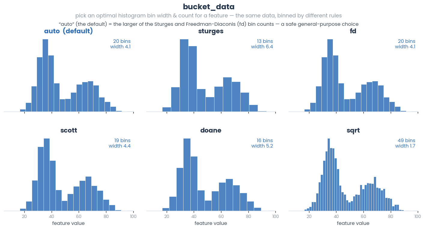
simba.utils.data.bucket_data(data: ndarray, method: typing_extensions.Literal['fd', 'doane', 'auto', 'scott', 'stone', 'rice', 'sturges', 'sqrt'] = 'auto') → Tuple[float, int][source]

Computes the optimal bin count and bin width non-heuristically using specified method.

Parameters

data (np.ndarray) – 1D array of numerical data.
method (np.ndarray) – The method to compute optimal bin count and bin width. These methods differ in how they estimate the optimal bin count and width. Defaults to ‘auto’, which represents the maximum of the Sturges and Freedman-Diaconis estimators. Available methods are ‘fd’, ‘doane’, ‘auto’, ‘scott’, ‘stone’, ‘rice’, ‘sturges’, ‘sqrt’.

Returns

A tuple containing the optimal bin width and bin count.

Return type

Tuple[float, int]

Example

>>> data = np.random.randint(low=1, high=1000, size=(1, 100))
>>> bucket_data(data=data, method='fd')
>>> (190.8, 6)
>>> bucket_data(data=data, method='doane')
>>> (106.0, 10)

simba.utils.data.bucket_data_mp(data: ndarray, method: typing_extensions.Literal['fd', 'doane', 'auto', 'scott', 'stone', 'rice', 'sturges', 'sqrt'] = 'auto', n_jobs: Optional[int] = -1) → Tuple[ndarray, ndarray][source]

Compute histogram bin edges for many inputs in parallel using CPU with Joblib.

Parameters

data – 2D input arrays for which to calculate histogram bin edges.
method (np.ndarray) – The method to compute optimal bin count and bin width. These methods differ in how they estimate the optimal bin count and width. Defaults to ‘auto’, which represents the maximum of the Sturges and Freedman-Diaconis estimators. Available methods are ‘fd’, ‘doane’, ‘auto’, ‘scott’, ‘stone’, ‘rice’, ‘sturges’, ‘sqrt’.
n_jobs – Number of CPU cores to use for parallelism (-1 uses all available cores).

Returns Tuple[float, int]

A tuple containing the optimal bin width and bin count.

simba.utils.data.center_rotation_warpaffine_vectors(rotation_vectors: ndarray, centers: ndarray)[source]: Create WarpAffine vectors for rotating a video around the center. These are used for egocentric alignment of video.

Note

rotation_vectors and centers are returned by simba.utils.data.egocentrically_align_pose(), or simba.utils.data.egocentrically_align_pose_numba() results are used within e.g., :func:`simba.video_processors.egocentric_video_rotator.EgocentricVideoRotator

simba.utils.data.convert_roi_definitions(roi_definitions_path: Union[str, PathLike], save_dir: Union[str, PathLike]) → None[source]

Helper to convert SimBA ROI_definitions.h5 file into human-readable CSV format.

Parameters

roi_definitions_path (Union[str, os.PathLike]) – Path to SimBA ROI_definitions.h5 on disk.
save_dir (Union[str, os.PathLike]) – Directory location where the output data should be stored

simba.utils.data.create_color_palette(pallete_name: str, increments: int, as_rgb_ratio: Optional[bool] = False, as_hex: Optional[bool] = False, as_int: Optional[bool] = False) → List[Union[str, float]][source]

Create a list of colors in RGB from specified color palette.

Parameters

pallete_name (str) – Palette name (e.g., jet)
increments (int) – Numbers of colors in the color palette to create.
as_rgb_ratio (Optional[bool]) – Return RGB to ratios. Default: False
as_hex (Optional[bool]) – Return values as HEX. Default: False
as_int (Optional[bool]) – Return RGB values as integers rather than float if possible. Default: False

Note

If both as_rgb_ratio and as_hex, HEX values will be returned.

Returns: Color palette values.
Return type: List[Union[str, float]]
Example

>>> create_color_palette(pallete_name='jet', increments=3)
>>> [[127.5, 0.0, 0.0], [255.0, 212.5, 0.0], [0.0, 229.81481481481478, 255.0], [0.0, 0.0, 127.5]]
>>> create_color_palette(pallete_name='jet', increments=3, as_rgb_ratio=True)
>>> [[0.5, 0.0, 0.0], [1.0, 0.8333333333333334, 0.0], [0.0, 0.0.9012345679012345, 1.0], [0.0, 0.0, 0.5]]
>>> create_color_palette(pallete_name='jet', increments=3, as_hex=True)
>>> ['#800000', '#ffd400', '#00e6ff', '#000080']

simba.utils.data.create_color_palettes(no_animals: int, map_size: int, cmaps: Optional[List[str]] = None) → List[List[int]][source]

Create list of lists of bgr colors, one for each animal. Each list is pulled from a different palette matplotlib color map.

Parameters

no_animals (int) – Number of different palette lists
map_size (int) – Number of colors in each created palette.

Returns

BGR colors

Return type

List[List[int]]

Example

>>> create_color_palettes(no_animals=2, map_size=2)
>>> [[[255.0, 0.0, 255.0], [0.0, 255.0, 255.0]], [[102.0, 127.5, 0.0], [102.0, 255.0, 255.0]]]

simba.utils.data.detect_bouts(data_df: DataFrame, target_lst: Union[List[str], str], fps: Union[int, float]) → DataFrame[source]

Detect behavior “bouts” (e.g., continous sequence of classified behavior-present frames) for specified classifiers.

Note

Can be any field of boolean type. E.g., target_lst = [‘Inside_ROI_1`] also works for bouts inside ROI shape.

See also

For multi-class Boolean classifiers, see simba.utils.data.detect_bouts_multiclass().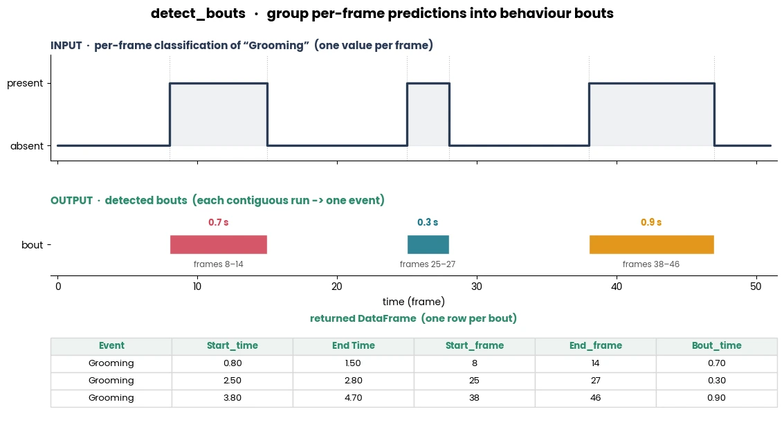

Parameters

data_df (pd.DataFrame) – Dataframe with fields representing classifications in boolean type.
target_lst (Union[List[str], str]) – Classifier names. E.g., as list or a single [‘Attack’, ‘Sniffing’, ‘Grooming’] string value ‘Attack’. Can be any boolean column name.
fps (Union[int, float]) – The fps of the input video.

Returns

Dataframe where bouts are represented by rows and fields are represented by ‘Event type ‘, ‘Start time’, ‘End time’, ‘Start frame’, ‘End frame’, ‘Bout time’

Return type

pd.DataFrame

Example

>>> data_df = read_df(file_path='tests/data/test_projects/two_c57/project_folder/csv/machine_results/Together_1.csv', file_type='csv')
>>> detect_bouts(data_df=data_df, target_lst=['Attack', 'Sniffing'], fps=25)
>>>     'Event'  'Start_time'  'End Time'  'Start_frame'  'End_frame'  'Bout_time'
>>> 0   'Attack'    5.03          5.33          151        159            0.30
>>> 1   'Attack'    5.87          6.23          176        186            0.37
>>> 2  'Sniffing'   3.47          3.83          104        114            0.37

simba.utils.data.detect_bouts_multiclass(data: DataFrame, target: str, fps: int = 1, classifier_map: Optional[Dict[int, str]] = None) → DataFrame[source]

Detect bouts in a multiclass time series dataset and return the bout event types, their start times, end times and duration.

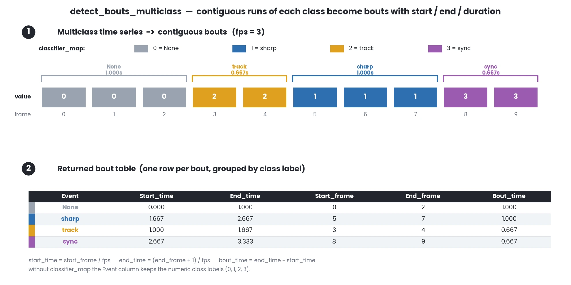
See also

For single class Boolean classifiers, see simba.utils.data.detect_bouts().

Parameters

data (pd.DataFrame) – A Pandas DataFrame containing multiclass time series data.
target (str) – Name of the target column in data.
fps (int) – Frames per second of the video used to collect data. Default is 1.
classifier_map (Dict[int, str]) – A dictionary mapping class labels to their names. Used to replace numeric labels with descriptive names. If None, then numeric event labels are kept.

Returns

Dataframe where bouts are represented by rows and fields are represented by ‘Event type ‘, ‘Start time’, ‘End time’, ‘Start frame’, ‘End frame’, ‘Bout time’

Return type

pd.DataFrame

Example

>>> df = pd.DataFrame({'value': [0, 0, 0, 2, 2, 1, 1, 1, 3, 3]})
>>> detect_bouts_multiclass(data=df, target='value', fps=3, classifier_map={0: 'None', 1: 'sharp', 2: 'track', 3: 'sync'})
>>>    'Event'  'Start_time'  'End_time'  'Start_frame'  'End_frame'  'Bout_time'
>>> 0   'None'    0.000000  1.000000          0.0        2.0   1.000000
>>> 1   'sharp'   1.666667  2.666667          5.0        7.0   1.000000
>>> 2   'track'   1.000000  1.666667          3.0        4.0   0.666667
>>> 3   'sync '   2.666667  3.333333          8.0        9.0   0.666667

simba.utils.data.df_smoother(data: DataFrame, fps: float, time_window: int, source: Optional[str] = '', std: Optional[int] = 5, method: Optional[typing_extensions.Literal['bartlett', 'blackman', 'boxcar', 'cosine', 'gaussian', 'hamming', 'exponential']] = 'gaussian') → DataFrame[source]

Smooth the data in a DataFrame using a specified window function.

This function applies a rolling window smoothing operation to the data in the DataFrame. The type of window function and the standard deviation for the smoothing can be specified. The window size is determined based on the frame rate per second (fps) and the time window.

See also

For low-pass Fourier smoothing, see simba.utils.data.fft_lowpass_filter(). For Savitzky-Golay smoothing, see simba.utils.data.savgol_smoother().

Parameters

data (pd.DataFrame) – The input data to be smoothed.
fps (float) – The frame rate per second of the data.
time_window (int) – The time window in milliseconds over which to apply the smoothing.
source (Optional[str]) – An optional string indicating the source of the data, used for logging and informative error messages.
std (Optional[int]) – The standard deviation for the window function, used when the method is ‘gaussian’.
method (Optional[Literal['bartlett', 'blackman', 'boxcar', 'cosine', 'gaussian', 'hamming', 'exponential']]) – The type of window function to use for smoothing. Default ‘gaussian’.

Return pd.DataFrame

The smoothed DataFrame.

simba.utils.data.egocentric_frm_rotator(frames: ndarray, rotation_matrices: ndarray, interpolate: Optional[bool] = True) → ndarray[source]

Rotates a sequence of frames using the provided rotation matrices in an egocentric manner using acceleration through numba JIT.

Applies a geometric transformation to each frame in the input sequence based on its corresponding rotation matrix. The transformation includes rotation and translation, followed by bilinear interpolation to map pixel values from the source frame to the output frame.

Note

To create rotation matrices, see simba.utils.data.center_rotation_warpaffine_vectors() and simba.utils.data.align_target_warpaffine_vectors()

Parameters

frames (np.ndarray) – A 4D array of shape (N, H, W, C)
rotation_matrices (np.ndarray) – A 3D array of shape (N, 3, 3), where each 3x3 matrix represents an affine transformation for a corresponding frame. The matrix should include rotation and translation components.

Returns

A 4D array of shape (N, H, W, C), representing the warped frames after applying the transformations. The shape matches the input frames.

Return type

np.ndarray

Example

>>> DATA_PATH = r"/mnt/c/Users/sroni/OneDrive/Desktop/rotate_ex/data/501_MA142_Gi_Saline_0513.csv"
>>> VIDEO_PATH = r"/mnt/c/Users/sroni/OneDrive/Desktop/rotate_ex/videos/501_MA142_Gi_Saline_0513.mp4"
>>> SAVE_PATH = r"/mnt/c/Users/sroni/OneDrive/Desktop/rotate_ex/videos/501_MA142_Gi_Saline_0513_rotated.mp4"
>>> ANCHOR_LOC = np.array([300, 300])
>>>
>>> df = read_df(file_path=DATA_PATH, file_type='csv')
>>> bp_cols = [x for x in df.columns if not x.endswith('_p')]
>>> data = df[bp_cols].values.reshape(len(df), int(len(bp_cols)/2), 2).astype(np.int64)
>>> data, centers, rotation_matrices = egocentrically_align_pose(data=data, anchor_1_idx=6, anchor_2_idx=2, anchor_location=ANCHOR_LOC, direction=180)
>>> imgs = read_img_batch_from_video_gpu(video_path=VIDEO_PATH, start_frm=0, end_frm=100)
>>> imgs = np.stack(list(imgs.values()), axis=0)
>>>
>>> rot_matrices_center = center_rotation_warpaffine_vectors(rotation_vectors=rotation_matrices, centers=centers)
>>> rot_matrices_align = align_target_warpaffine_vectors(centers=centers, target=ANCHOR_LOC)
>>>
>>> imgs_centered = egocentric_frm_rotator(frames=imgs, rotation_matrices=rot_matrices_center)
>>> imgs_out = egocentric_frm_rotator(frames=imgs_centered, rotation_matrices=rot_matrices_align)

simba.utils.data.egocentrically_align_pose(data: ndarray, anchor_1_idx: int, anchor_2_idx: int, anchor_location: ndarray, direction: int) → Tuple[ndarray, ndarray, ndarray][source]

Aligns a set of 2D points egocentrically based on two anchor points and a target direction.

Rotates and translates a 3D array of 2D points (e.g., time-series of frame-wise data) such that one anchor point is aligned to a specified location, and the direction between the two anchors is aligned to a target angle.

See also

For numba acceleration, see simba.utils.data.egocentrically_align_pose_numba(). To align both pose and video, see simba.data_processors.egocentric_aligner.EgocentricalAligner(). To egocentrically rotate video, see simba.video_processors.egocentric_video_rotator.EgocentricVideoRotator()

Parameters

data (np.ndarray) – A 3D array of shape (num_frames, num_points, 2) containing 2D points for each frame. Each frame is represented as a 2D array of shape (num_points, 2), where each row corresponds to a point’s (x, y) coordinates.
anchor_1_idx (int) – The index of the first anchor point in data used as the center of alignment. This body-part will be placed in the center of the image.
anchor_2_idx (int) – The index of the second anchor point in data used to calculate the direction vector. This bosy-part will be located direction degrees from the anchor_1 body-part.
direction (int) – The target direction in degrees to which the vector between the two anchors will be aligned.
anchor_location (np.ndarray) – A 1D array of shape (2,) specifying the target (x, y) location for anchor_1_idx after alignment.

Returns

A tuple containing the rotated data, and variables required for also rotating the video using the same rules: - aligned_data: A 3D array of shape (num_frames, num_points, 2) with the aligned 2D points. - centers: A 2D array of shape (num_frames, 2) containing the original locations of anchor_1_idx in each frame before alignment. - rotation_vectors: A 3D array of shape (num_frames, 2, 2) containing the rotation matrices applied to each frame.

Return type

Tuple[np.ndarray, np.ndarray, np.ndarray]

Example

>>> data = np.random.randint(0, 500, (100, 7, 2))
>>> anchor_1_idx = 5 # E.g., the animal tail-base is the 5th body-part
>>> anchor_2_idx = 7 # E.g., the animal nose is the 7th row in the data
>>> anchor_location = np.array([250, 250]) # the tail-base (index 5) is placed at x=250, y=250 in the image.
>>> direction = 90 # The nose (index 7) will be placed in direction 90 degrees (S) relative to the tailbase.
>>> results, centers, rotation_vectors = egocentrically_align_pose(data=data, anchor_1_idx=anchor_1_idx, anchor_2_idx=anchor_2_idx, direction=direction)

simba.utils.data.egocentrically_align_pose_numba(data: ndarray, anchor_1_idx: int, anchor_2_idx: int, direction: int, anchor_location: ndarray) → Tuple[ndarray, ndarray, ndarray][source]

Aligns a set of 2D points egocentrically based on two anchor points and a target direction.

Rotates and translates a 3D array of 2D points (e.g., time-series of frame-wise data) such that one anchor point is aligned to a specified location, and the direction between the two anchors is aligned to a target angle.

EXPECTED RUNTIMES
FRAMES (MILLIONS)	NUMBA TIME (S)	NUMBA TIME (STEV)	NUMPY TIME (S)	NUMPY TIME (STEV)
1	0.733	0.006	10.138	0.459
2	1.474	0.004	16.894	0.264
4	2.969	0.032	33.813	0.371
8	5.991	0.061	73.434	0.526
16	12.123	0.215	134.028	0.858
32	23.844	0.105	270.435	1.379
64	48.296	0.034	540.896	1.781
7 BODY-PARTS PER FRAME
3 ITERATIONS

See also

For numpy function, see simba.utils.data.egocentrically_align_pose(). To align both pose and video, see simba.data_processors.egocentric_aligner.EgocentricalAligner(). To egocentrically rotate video, see simba.video_processors.egocentric_video_rotator.EgocentricVideoRotator()

Parameters

data (np.ndarray) – A 3D array of shape (num_frames, num_points, 2) containing 2D points for each frame. Each frame is represented as a 2D array of shape (num_points, 2), where each row corresponds to a point’s (x, y) coordinates.
anchor_1_idx (int) – The index of the first anchor point in data used as the center of alignment. This body-part will be placed in the center of the image.
anchor_2_idx (int) – The index of the second anchor point in data used to calculate the direction vector. This bosy-part will be located direction degrees from the anchor_1 body-part.
direction (int) – The target direction in degrees to which the vector between the two anchors will be aligned.
anchor_location (np.ndarray) – A 1D array of shape (2,) specifying the target (x, y) location for anchor_1_idx after alignment.

Returns

A tuple containing the rotated data, and variables required for also rotating the video using the same rules: - aligned_data: A 3D array of shape (num_frames, num_points, 2) with the aligned 2D points. - centers: A 2D array of shape (num_frames, 2) containing the original locations of anchor_1_idx in each frame before alignment. - rotation_vectors: A 3D array of shape (num_frames, 2, 2) containing the rotation matrices applied to each frame.

Return type

Tuple[np.ndarray, np.ndarray, np.ndarray]

Example

>>> data = np.random.randint(0, 500, (100, 7, 2))
>>> anchor_1_idx = 5 # E.g., the animal tail-base is the 5th body-part
>>> anchor_2_idx = 7 # E.g., the animal nose is the 7th row in the data
>>> anchor_location = np.array([250, 250]) # the tail-base (index 5) is placed at x=250, y=250 in the image.
>>> direction = 90 # The nose (index 7) will be placed in direction 90 degrees (S) relative to the tailbase.
>>> results, centers, rotation_vectors = egocentrically_align_pose_numba(data=data, anchor_1_idx=anchor_1_idx, anchor_2_idx=anchor_2_idx, direction=direction)

simba.utils.data.fast_mean_rank(data: ndarray, descending: Optional[bool] = True) → ndarray[source]

Jitted helper to rank values in 1D array using mean method.

See also

simba.utils.data.fast_minimum_rank()

Parameters

data (np.ndarray) – 1D array of feature values.
descending (bool) – If True, ranks returned where low values get a high rank. If False, low values get a low rank. Default: True.

Returns

1D array with the data values ranked indices.

Return type

np.ndarray

References

Modified from James Webber gist on GitHub.

Example

>>> data = np.array([1, 1, 3, 4, 5, 6, 7, 8, 9, 10])
>>> fast_mean_rank(data=data, descending=True)
>>> [9.5, 9.5, 8. , 7. , 6. , 5. , 4. , 3. , 2. , 1. ]

simba.utils.data.fast_minimum_rank(data: ndarray, descending: Optional[bool] = True) → ndarray[source]

Jitted helper to rank values in 1D array using minimum method.

See also

simba.utils.data.fast_mean_rank()

Parameters

data (np.ndarray) – 1D array of feature values.
descending (bool) – If True, ranks returned where low values get a high rank. If False, low values get a low rank. Default: True.

Returns

1D array with the data values ranked indices.

Return type

np.ndarray

References

Jérôme Richard on StackOverflow.

Example

>>> data = np.array([1, 1, 3, 4, 5, 6, 7, 8, 9, 10])
>>> fast_minimum_rank(data=data, descending=True)
>>> [9, 9, 8, 7, 6, 5, 4, 3, 2, 1]
>>> fast_minimum_rank(data=data, descending=False)
>>> [ 1,  1,  3,  4,  5,  6,  7,  8,  9, 10]

simba.utils.data.fft_lowpass_filter(data: ndarray, cut_off: float = 0.1) → ndarray[source]

Apply FFT-based lowpass filter to 1D or 2D data.

See also

For Savitzky-Golay smoothing, see simba.utils.data.savgol_smoother(). For ‘bartlett’, ‘blackman’, ‘boxcar’, ‘cosine’, ‘gaussian’, ‘hamming’, ‘exponential’ smoothing, see func:simba.utils.data.df_smoother.

Parameters

data (np.ndarray) – Input data array (1D or 2D)
cut_off (float) – Cutoff frequency as fraction of Nyquist frequency (0 < cut_off < 1)

Return np.ndarray

Filtered data with same shape and dtype as input

Example

>>> from simba.utils.read_write import read_df
>>> IN_PATH = r"C:/troubleshooting/RAT_NOR/project_folder/csv/outlier_corrected_movement_location/2022-06-20_NOB_DOT_4.csv"
>>> OUT_PATH = r"C:/troubleshooting/RAT_NOR/project_folder/csv/outlier_corrected_movement_location/2022-06-20_NOB_DOT_4_filtered.csv"
>>> df = read_df(file_path=IN_PATH)
>>> data = df.values
>>> x = fft_lowpass_filter(data=data, cut_off=0.1)

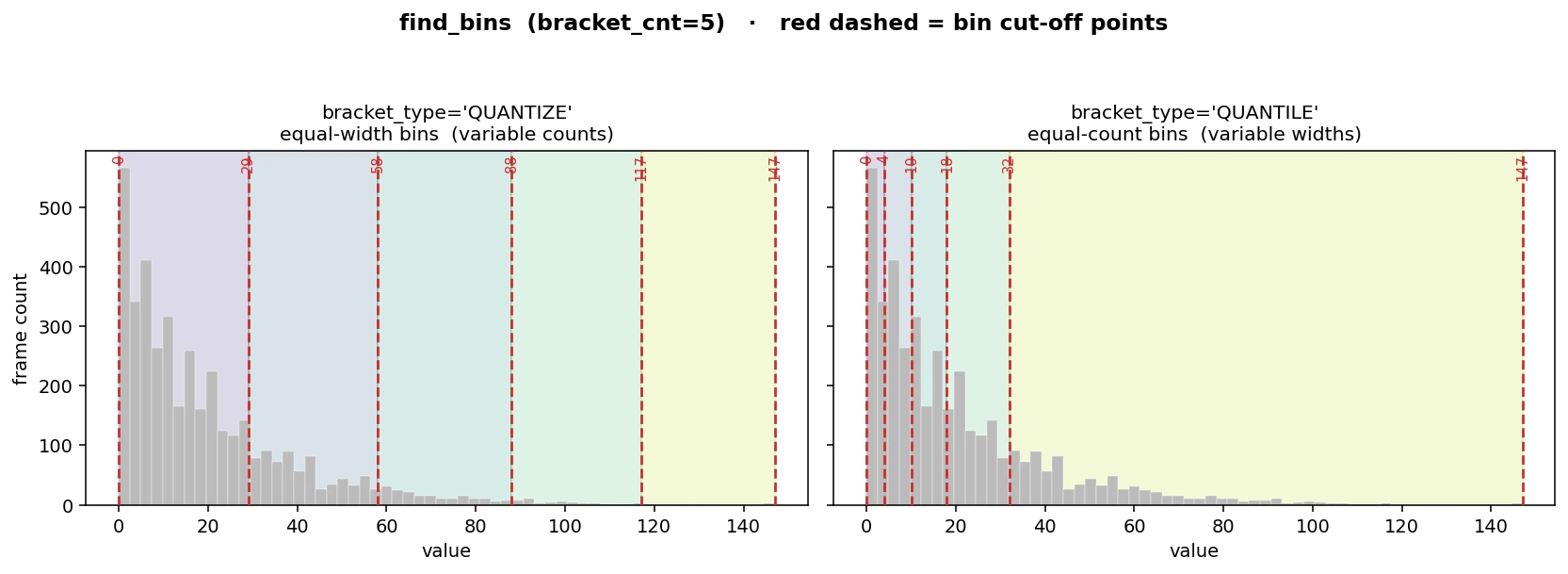
simba.utils.data.find_bins(data: Dict[str, List[int]], bracket_type: typing_extensions.Literal['QUANTILE', 'QUANTIZE'], bracket_cnt: int, normalization_method: typing_extensions.Literal['ALL VIDEOS', 'BY VIDEO']) → Dict[str, ndarray][source]

Helper to find bin cut-off points.

Parameters

data (dict) – Dictionary with video names as keys and list of values of size len(frames).
bracket_type (Literal[str]) – ‘QUANTILE’ or ‘QUANTIZE’
bracket_cnt (str) – Number of bins.
normalization_method (str) – Create bins based on data in all videos (“ALL VIDEOS”) or create different bins per video (‘BY VIDEO’)

Returns dict

The videos as keys and bin cut off points as array of size len(bracket_cnt) x 2.

simba.utils.data.find_frame_numbers_from_time_stamp(start_time: str, end_time: str, fps: int) → List[int][source]

Given start and end timestamps in HH:MM:SS formats and the fps, return the frame numbers representing the time period.

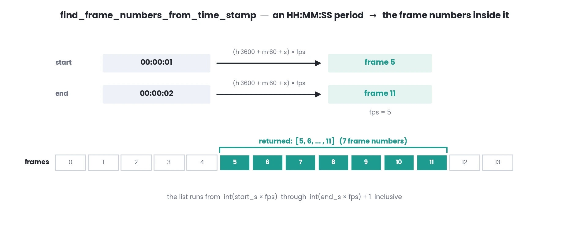
Note

For the converse (find frame numbers from start and in HH:MM:SS format), use func:simba.utils.read_write.find_time_stamp_from_frame_numbers.

Parameters

start_time (str) – Period start time in HH:MM:SS format.
end_time (str) – Period end time in HH:MM:SS format.
fps (int) – Framerate of the video.

Returns

Frame numbers within the period.

Return type

List[int]

Example

>>> find_frame_numbers_from_time_stamp(start_time='00:00:00', end_time='00:00:01', fps=10)
>>> [0, 1, 2, 3, 4, 5, 6, 7, 8, 9, 10]

simba.utils.data.find_ranked_colors(data: Dict[Any, float], palette: str, as_hex: bool = False, as_rgb_ratio: bool = False, reverse: bool = True) → Dict[str, Union[Tuple[int], str]][source]

Find ranked colors for a given data dictionary values based on a specified color palette.

The key with the highest value in the data dictionary is assigned the most intense palette color, while the key with the lowest value in the data dictionary is assigned the least intense palette color.

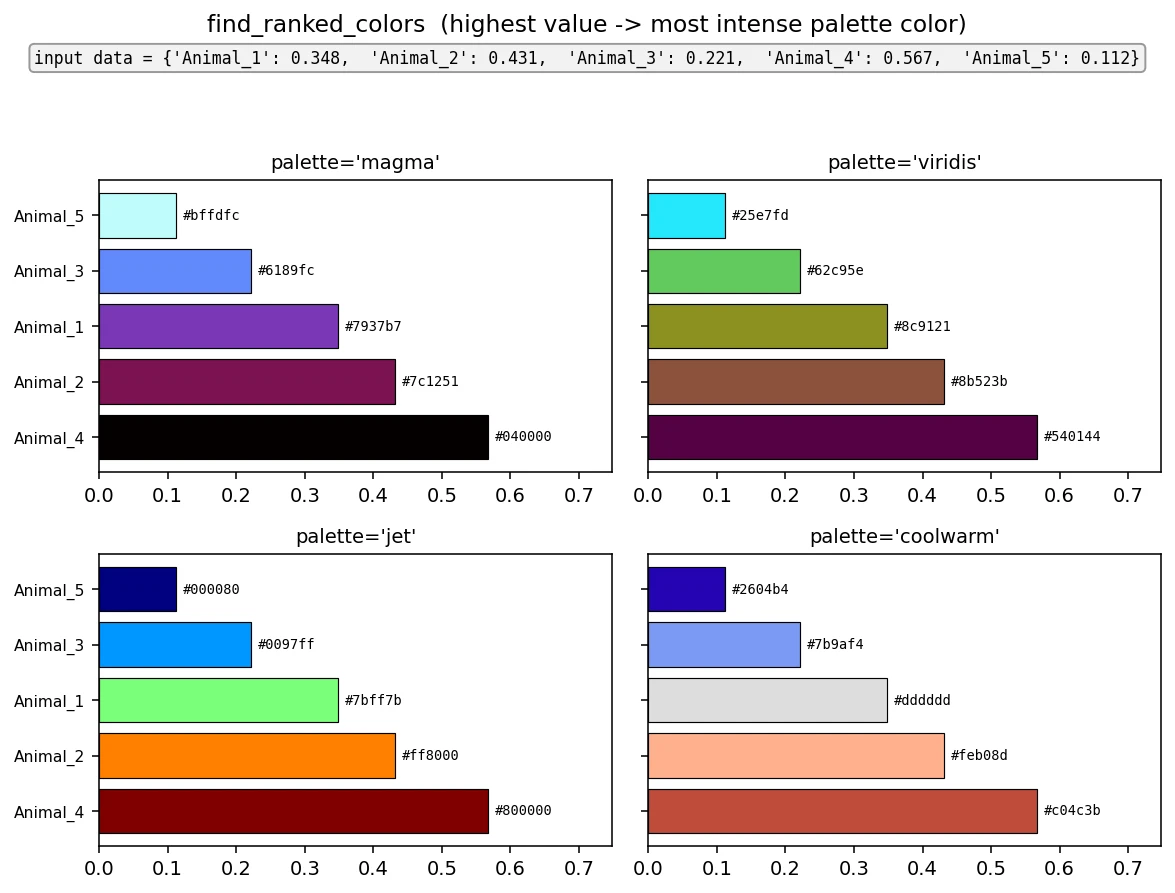
Parameters

data – A dictionary where keys are labels and values are numerical scores.
palette – A string representing the name of the color palette to use (e.g., ‘magma’).
as_hex – If True, return colors in hexadecimal format; if False, return as RGB tuples. Default is False.

Returns

A dictionary where keys are labels and values are corresponding colors based on ranking.

Return type

Dict[str, Union[Tuple[int], str]]

Examples

>>> data = {'Animal_1': 0.34786870380536705, 'Animal_2': 0.4307923198152757, 'Animal_3': 0.221338976379357}
>>> find_ranked_colors(data=data, palette='magma', as_hex=True)
>>> {'Animal_2': '#040000', 'Animal_1': '#7937b7', 'Animal_3': '#bffdfc'}

simba.utils.data.freedman_diaconis(data: ndarray) → Tuple[float, int][source]

Use Freedman-Diaconis rule to compute optimal count of histogram bins and their width.

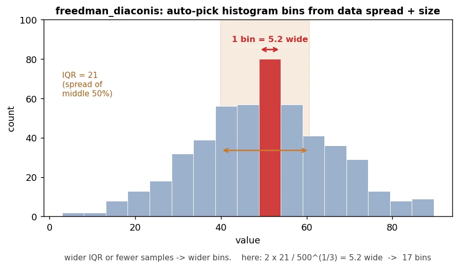
Note

Can also use simba.utils.data.bucket_data passing method fd.

Parameters

data (np.ndarray) – 1d array with values to compute optimal bins for.

Returns

Tuple representing the optimal count of histogram bins and their width.

Return type

Tuple[float, int]

References

2: Reference freedman_diaconis.

simba.utils.data.get_confusion_matrix(x: ndarray, y: ndarray) → ndarray[source]

Compute a confusion matrix

Note

Adapted from mucunwuxian’s Stack Overflow answer: https://stackoverflow.com/a/67747070

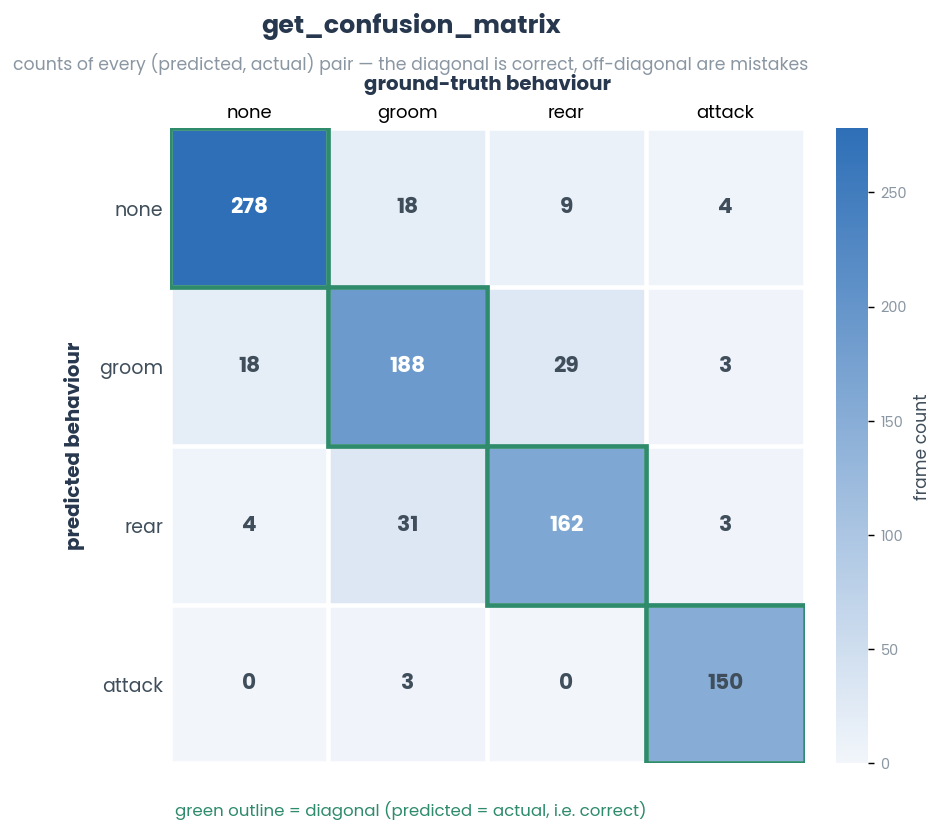
Parameters

x (np.ndarray) – Predicted cluster labels (1D array of integers).
y (np.ndarray) – Ground truth class labels (1D array of integers, same length as x).

Returns

A 2D confusion matrix of shape (n_labels, n_labels), where entry (i, j) is the number of times label i in x coincided with label j in y.

Return type

np.ndarray

Example

>>> x = np.random.randint(0, 5, (100000,))
>>> y = np.random.randint(0, 5, (100000,))
>>> c = get_confusion_matrix(x=x, y=y)

simba.utils.data.get_cpu_pool(core_cnt: int = -1, maxtasksperchild: int = 8000, context: Optional[typing_extensions.Literal['fork', 'spawn', 'forkserver']] = None, verbose: bool = True, source: Optional[str] = None) → Pool[source]

Creates and returns a multiprocessing.Pool instance with platform-appropriate defaults and validation.

Parameters

core_cnt (int) – Number of worker processes. -1 uses all available cores. Default: -1.
maxtasksperchild (int) – Maximum number of tasks a worker process can complete before being replaced. Default: From Defaults.MAXIMUM_MAX_TASK_PER_CHILD.
context (Optional[Literal['fork', 'spawn', 'forkserver']]) – Multiprocessing start method. None uses platform default. Default: None.
verbose (bool) – If True, prints pool creation message with timestamp. Default: True.
source (Optional[str]) – Optional identifier string for logging purposes (e.g., ‘VideoProcessor’). Default: None.

Returns

Configured multiprocessing.Pool instance.

Return type

multiprocessing.Pool

Example

>>> pool = get_cpu_pool(core_cnt=4, source='FeatureExtractor')
>>> pool = get_cpu_pool(core_cnt=-1, context='spawn', verbose=True)
>>> pool = get_cpu_pool(core_cnt=8, maxtasksperchild=100, source='VideoProcessor')

simba.utils.data.get_library_version(library_name: str, raise_error: bool = False) → Union[str, bool][source]

Get the version installed package in python environment.

Parameters: library_name (str) – Name of library.
Return str: Library version name, if installed
Example

>>> get_library_version(library_name='sklearn')
>>> 0.22.2

simba.utils.data.get_mode(x: ndarray) → Union[float, int][source]

Get the mode (most frequent value) within an array

Parameters: x (np.ndarray) – 1d array of numerics.
Returns: The mode of x.
Rtype Union[float, int]

simba.utils.data.hist_1d(data: ndarray, bins: int, range: ndarray)[source]

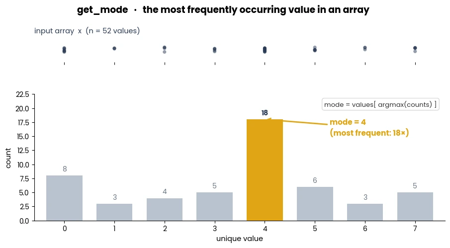
simba.utils.data.hist_1d_mp(data: ndarray, bin_counts: ndarray, bin_widths: ndarray, normalize: Optional[bool] = False) → List[source]

Jitted helper to compute 1D histograms with counts or rations (if normalize is True) for a 2D dataset

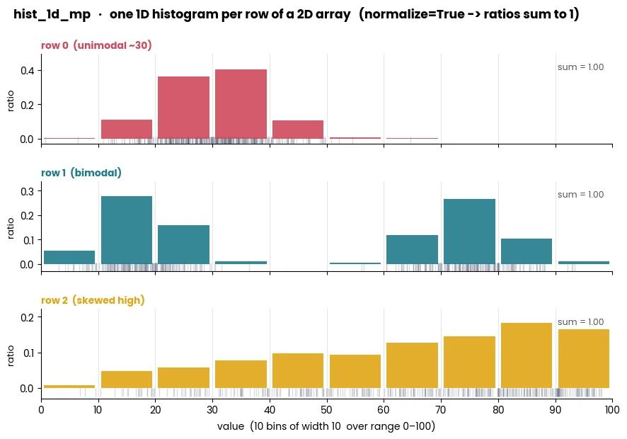
Note

For non-heuristic rules for bin counts and bin ranges, see simba.data.freedman_diaconis or simba.data.bucket_data``.

For computing a single 1D histogram from 1d data, use : func: hist_1d_

Parameters

data (np.ndarray) – 2d array containing feature values. The data in each row will be binned seperately.
bin_count (int) – The number of bins.
range (np.ndarray) – 1d array with two values representing minimum and maximum value to bin.
normalize (Optional[bool]) – If True, then the counts are returned as a ratio of all values. If False, then the raw counts. Pass normalize as True if the datasets are unequal counts. Default: True.

Returns

A numba list of list of same size as data.shape[0]

Return type

typed.List

Example

>>> data = np.random.randint(0, 100, (900, 300))
>>> bin_counts, bin_widths = bucket_data_mp(data=data)
>>> r = hist_1d_mp(data=data, bin_counts=bin_counts, bin_widths=bin_widths, normalize=True)

simba.utils.data.interpolate_color_palette(start_color: Tuple[int, int, int], end_color: Tuple[int, int, int], n: Optional[int] = 10) → List[Tuple[int, int, int]][source]

Generate a list of colors interpolated between two passed RGB colors.

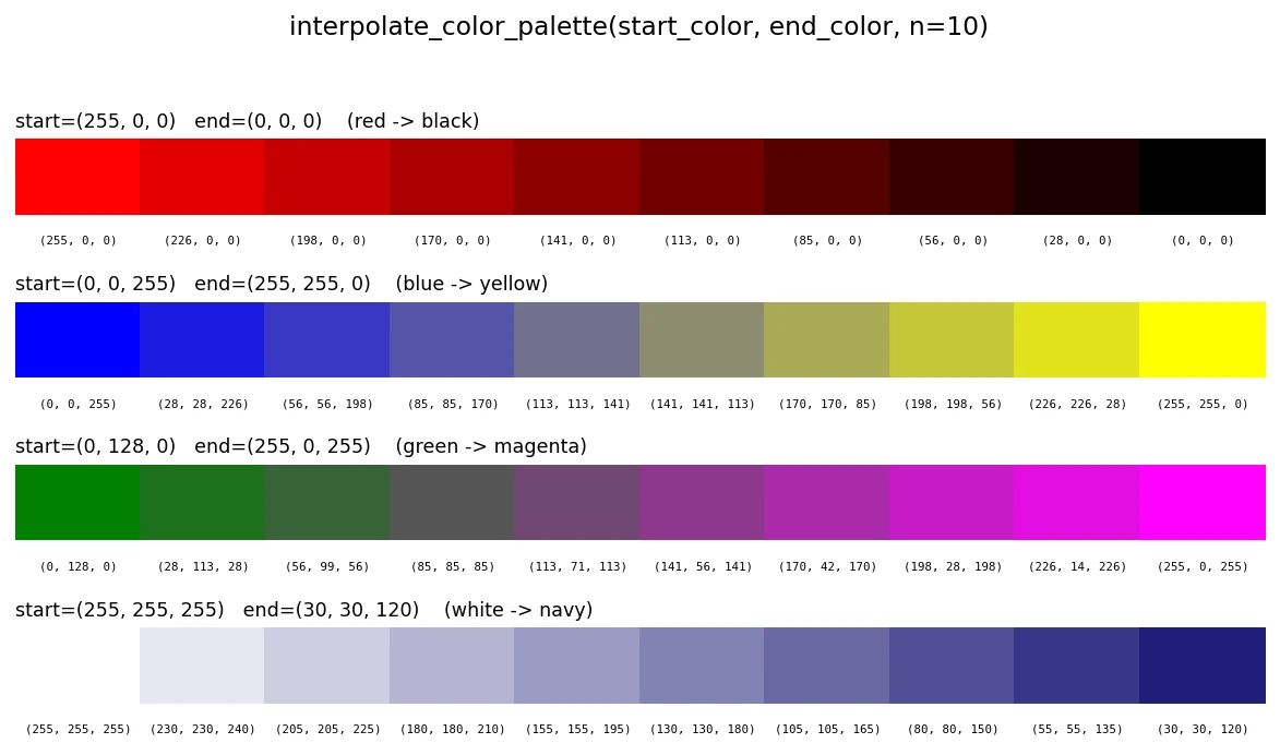
Parameters

start_color – Tuple of RGB values for the start color.
end_color – Tuple of RGB values for the end color.
n – Number of colors to generate.

Returns

List of interpolated RGB colors.

Return type

List[Tuple[int, int, int]]

Example

>>> red, black = (255, 0, 0), (0, 0, 0)
>>> colors = interpolate_color_palette(start_color=red, end_color=black, n = 10)

simba.utils.data.plug_holes_shortest_bout(data_df: DataFrame, clf_name: str, fps: float, shortest_bout: int) → DataFrame[source]

Removes behavior “bouts” that are shorter than the minimum user-specified length within a dataframe.

Note

In the initial step the function looks for behavior “interuptions” that are the length of the shortest_bout or shorter. I.e., these are 0 sequences that are the length of the shortest_bout or shorter with trailing and leading 1`s. These interuptions are filled with `1`s. Next, the behavioral bouts shorter than the `shortest_bout are removed. This operations are perfomed as it helps in preserving longer sequences of the desired behavior, ensuring they aren’t fragmented by brief interruptions.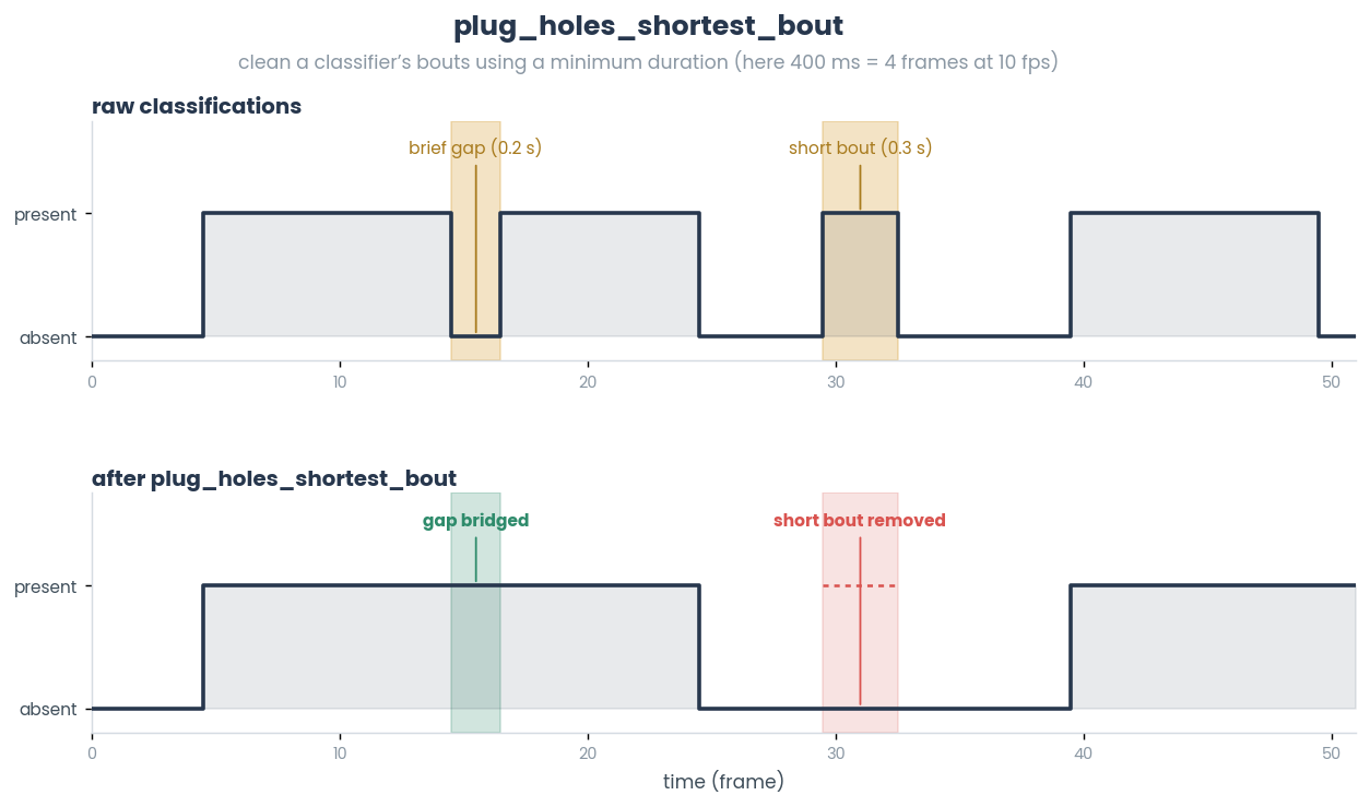

Parameters

data_df (pd.DataFrame) – Pandas Dataframe with classifier prediction data.
clf_name (str) – Name of the classifier field of list of names of classifier fields
fps (int) – The fps of the input video.
shortest_bout (int) – The shortest valid behavior boat in milliseconds.

Returns

Dataframe where behavior bouts with invalid lengths have been removed (< shortest_bout)

Return type

pd.DataFrame

Example

>>>  data_df = pd.DataFrame(data=[1, 0, 1, 1, 1], columns=['target'])
>>>  plug_holes_shortest_bout(data_df=data_df, clf_name='target', fps=10, shortest_bout=2000)
>>>         target
>>>    0       1
>>>    1       1
>>>    2       1
>>>    3       1
>>>    4       1

simba.utils.data.resample_geometry_vertices(vertices: Union[List[ndarray], ndarray], vertice_cnt: int) → ndarray[source]

Resample geometry vertices to a specified number of vertices in each polygon.

This function takes a list or a single array of 2D coordinates representing the vertices of polygons and resamples each polygon to have exactly vertice_cnt vertices. The resampling is done by interpolating the distances between consecutive vertices and then uniformly distributing the requested number of vertices along the perimeter of each polygon.

Parameters

np.ndarray] (Union[List[np.ndarray],) – A list of 2D coordinate arrays or a single 3D array representing the vertices of polygons. Each 2D array should have shape (n, 2), where n is the number of vertices.
vertice_cnt (int) – The target number of vertices for resampling in each polygon. This value should be at least 3.

Returns

A 3D array of shape (len(vertices), vertice_cnt, 2), where each 2D array in the result contains the resampled vertices of the corresponding polygon.

Return type

np.ndarray

simba.utils.data.run_user_defined_feature_extraction_class(file_path: Union[str, PathLike], config_path: Union[str, PathLike]) → None[source]

Loads and executes user-defined feature extraction class within .py file.

Parameters

file_path – Path to .py file holding user-defined feature extraction class.
config_path (str) – Path to SimBA project config file.

Warning

Legacy function. The GUI since 12/23 uses simba.utils.custom_feature_extractor.UserDefinedFeatureExtractor().

Note

Tutorial.

If the file_path contains multiple classes, then the first class will be used.

The user defined class needs to contain a config_path init argument.

If the feature extraction class contains a if __name__ == "__main__": entry point and uses argparse, then the custom feature extraction module will be executed through python subprocess.

Else, will be executed using sys.

I recommend using the if __name__ == "__main__: and subprocess alternative, as the feature extraction clas will be executed in a different thread and any multicore parallel processes within the user feature extraction class will not be throttled by the graphical interface mainloop.

Example

>>> run_user_defined_feature_extraction_class(config_path='/Users/simon/Desktop/envs/troubleshooting/circular_features_zebrafish/project_folder/project_config.ini', file_path='/Users/simon/Desktop/fish_feature_extractor_2023_version_5.py')
>>> run_user_defined_feature_extraction_class(config_path='/Users/simon/Desktop/envs/troubleshooting/piotr/project_folder/train-20231108-sh9-frames-with-p-lt-2_plus3-&3_best-f1.ini', file_path='/simba/misc/piotr.py')

simba.utils.data.sample_df_n_by_unique(df: DataFrame, field: str, n: int) → DataFrame[source]

Randomly sample at most N rows per unique value in specified field of a dataframe.

For example, sample 100 observation from each inferred cluster assignment.

Parameters

pd.DataFramedf – The dataframe to sample from.
field (str) – The column name in the DataFrame to use for sampling based on unique values.
n (int) – The maximum number of rows to sample for each unique value in the specified column.

:return A dataframe containing randomly sampled rows. :rtype: pd.DataFrame

simba.utils.data.savgol_smoother(data: Union[DataFrame, ndarray], fps: float, time_window: int, source: Optional[str] = '', mode: Optional[typing_extensions.Literal['mirror', 'constant', 'nearest', 'wrap', 'interp']] = 'nearest', polyorder: Optional[int] = 3) → Union[DataFrame, ndarray][source]

Apply Savitzky-Golay smoothing to the input data pose-estimation data

Applies the Savitzky-Golay filter to smooth the data in a DataFrame or a NumPy array. The filter smoothes the data using a polynomial of the specified order and a window size based on the frame rate per second (fps) and the time window.

See also

For ‘bartlett’, ‘blackman’, ‘boxcar’, ‘cosine’, ‘gaussian’, ‘hamming’, ‘exponential’ smoothing, see func:simba.utils.data.df_smoother. For low-pass Fourier smoothing, see simba.utils.data.fft_lowpass_filter().

Parameters

data (Union[pd.DataFrame, np.ndarray]) – The input data to be smoothed. Can be a pandas DataFrame or a 2D NumPy array.
fps (float) – The frame rate per second of the data.
time_window (int) – The time window in milliseconds over which to apply the smoothing.
source (Optional[str]) – An optional string indicating the source of the data, used for logging and informative error messages.
mode (Optional[Literal['mirror', 'constant', 'nearest', 'wrap', 'interp']]) – The mode parameter determines the behavior at the edges of the data. Options are:’mirror’, ‘constant’, ‘nearest’, ‘wrap’, ‘interp’. Default: ‘nearest’.
polyorder (Optional[int]) – The order of the polynomial used to fit the samples.

Return Union[pd.DataFrame, np.ndarray]

The smoothed data, returned as a DataFrame if the input was a DataFrame, or a NumPy array if the input was an array.

Example

>>> data = pd.read_csv('/Users/simon/Desktop/envs/simba/troubleshooting/two_black_animals_14bp/project_folder/csv/machine_results/Together_1.csv', index_col=0)
>>> savgol_smoother(data=data.values, fps=15, time_window=1000)

simba.utils.data.scale_pose_keypoints(keypoints: ndarray, original_size: Tuple[int, int], new_size: Tuple[int, int]) → ndarray[source]

Scale pose keypoints from original image dimensions to new image dimensions.

Parameters

keypoints (np.ndarray) – Nx2 array of (x, y) coordinates in pixel space, or 1D array of (x, y) for a single point.
original_size (Tuple[int, int]) – (width, height) of the original image.
new_size (Tuple[int, int]) – (width, height) of the target image.

Returns

Array of scaled (x, y) coordinates. Same shape as input (1D if input was 1D, else Nx2).

Example

>>> kp = np.array([[100, 200], [300, 400]])
>>> scale_pose_keypoints(kp, original_size=(640, 480), new_size=(320, 240))
>>> scale_pose_keypoints(np.array([100, 200]), original_size=(640, 480), new_size=(320, 240))

simba.utils.data.slice_roi_dict_for_video(data: Dict[str, DataFrame], video_name: str) → Tuple[Dict[str, DataFrame], List[str]][source]

Given a dictionary of dataframes representing different ROIs (created by simba.mixins.config_reader.ConfigReader.read_roi_data), retain only the ROIs belonging to the specified video.

Parameters

data (Dict[str, pd.DataFrame]) – Dictionary with Circle`, ``Polygon and Rectangle keys and dataframe values.
video_name (str) – Name of the vidio which ROIs should be sliced out.

Returns

Tuple with (i) a dictionary of the same shape as input data, and a list of the roi names for the sliced video.

Return type

Tuple[Dict[str, pd.DataFrame], List[str]]

simba.utils.data.slice_roi_dict_from_attribute(data: Dict[str, DataFrame], shape_names: Optional[List[str]] = None, video_names: Optional[List[str]] = None) → Tuple[Dict[str, DataFrame], List[str], int][source]

Filters ROI (Region of Interest) shape data based on provided shape names and/or video names.

Parameters

data (Dict[str, pd.DataFrame]) – A dictionary where keys are shape type strings (e.g., ‘Rectangles’, ‘Circles’, ‘Polygons’), and values are pandas DataFrames containing at least ‘Name’ and ‘Video’ columns. Obtained from ConfigReader.read_roi_data.
shape_names (Union[str, List[str]]) – A string or list of strings specifying ROI names to retain. If None, all names are kept.
video_names (Union[str, List[str]]) – A string or list of strings specifying video names to retain. If None, all videos are kept.

Returns

A dictionary of filtered DataFrames, one per shape type, with the index reset, the names of the ROIs, and the number of shapes returned.

Return type

Tuple[Dict[str, pd.DataFrame], List[str], int]

simba.utils.data.slp_to_df_convert(file_path: Union[str, PathLike], headers: List[str], joined_tracks: Optional[bool] = False, multi_index: Optional[bool] = True, drop_body_parts: Optional[List[str]] = None) → DataFrame[source]

Helper to convert .slp pose-estimation data in h5 format to pandas dataframe.

Parameters

file_path (Union[str, os.PathLike]) – Path to SLEAP H5 file on disk.
headers (List[str]) – List of strings representing output dataframe headers.
joined_tracks (bool) – If True, the h5 file has been created by joining multiple .slp files.
multi_index (bool) – If True, inserts multi-index place-holders in the output dataframe (used in SimBA data import).
drop_body_parts (Optional[List[str]]) – Body-parts that should be removed from the SLEAP H5 dataset before import into SimBA. Use the body-part names as defined in SLEAP. Default: None.

Raises

InvalidFileTypeError – If file_path is not a valid SLEAP H5 pose-estimation file.
DataHeaderError – If sleap file contains more or less body-parts than suggested by len(headers)

Return pd.DataFrame

With animal ID, Track ID and body-part names as columns.

Example

>>> headers = ['d_nose_1', 'd_neck_1', 'd_back_1', 'd_tail_1', 'nest_s_2', 'nest_cc_2', 'nest_cv_2', 'nest_cc_2', 'nest_csc_2', 'nest_cscd_2']
>>> new_headers = []
>>> for h in headers: new_headers.append(h + '_x'); new_headers.append(h + '_y'); new_headers.append(h + '_p')
>>> df = slp_to_df_convert(file_path='/Users/simon/Desktop/envs/troubleshooting/ryan/LBN4a_Ctrl_P05_1_2022-01-15_08-16-20c.h5', headers=new_headers, joined_tracks=True)

simba.utils.data.smooth_data_gaussian(config: ConfigParser, file_path: str, time_window_parameter: int) → None[source]

Perform Gaussian smoothing of pose-estimation data.

Important

Overwrites the input data with smoothened data.

Parameters

config (configparser.ConfigParser) – Parsed SimBA project_config.ini file.
file_path (str) – Path to pose estimation data.
time_window_parameter (int) – Gaussian rolling window size in milliseconds.

Example

>>> config = read_config_file(ini_path='/Users/simon/Desktop/envs/troubleshooting/Tests_022023/project_folder/project_config.ini')
>>> smooth_data_gaussian(config=config, file_path='/Users/simon/Desktop/envs/troubleshooting/Tests_022023/project_folder/csv/input_csv/Together_1.csv', time_window_parameter=500)

simba.utils.data.smooth_data_savitzky_golay(config: ConfigParser, file_path: Union[str, PathLike], time_window_parameter: int, overwrite: Optional[bool] = True) → None[source]

Perform Savitzky-Golay smoothing of pose-estimation data within a file.

Important

LEGACY: USE simba.utils.data.savgol_smoother instead.

Overwrites the input data with smoothened data.

Parameters

config (configparser.ConfigParser) – Parsed SimBA project_config.ini file.
file_path (str) – Path to pose estimation data.
time_window_parameter (int) – Savitzky-Golay rolling window size in milliseconds.
overwrite (bool) – If True, overwrites the input data. If False, returns the smoothened dataframe.

Example

>>> config = read_config_file(config_path='Tests_022023/project_folder/project_config.ini')
>>> smooth_data_savitzky_golay(config=config, file_path='Tests_022023/project_folder/csv/input_csv/Together_1.csv', time_window_parameter=500)

simba.utils.data.terminate_cpu_pool(pool: Pool, force: bool = False, verbose: bool = True, source: Optional[str] = None) → None[source]

Safely terminates a multiprocessing.Pool instance with optional graceful shutdown.

Note

If pool is None or invalid, function returns without action. Exceptions during termination are silently caught.

Parameters

pool (multiprocessing.pool.Pool) – The multiprocessing pool to terminate. If None, function returns without action.
force (bool) – If True, skips graceful shutdown (close/join) and immediately terminates. Default: False.
verbose (bool) – If True, prints termination message with timestamp. Default: True.
source (Optional[str]) – Optional identifier string for logging purposes (e.g., ‘VideoProcessor’). Default: None.

Example

>>> import multiprocessing
>>> pool = multiprocessing.Pool(4)
>>> terminate_cpu_pool(pool=pool, force=False, verbose=True, source='FeatureExtractor')

SimBA Enumerals

class simba.utils.enums.ConfigKey(value)[source]

Bases: Enum

An enumeration.

ANIMAL_CNT = 'animal_no'

BODYPART_DIRECTION_VALUE = 'bodypart_direction'

CREATE_ENSEMBLE_SETTINGS = 'create ensemble settings'

DIRECTIONALITY_SETTINGS = 'Directionality settings'

DISPLAY_SETTINGS = 'DISPLAY SETTINGS'

DISTANCE_MM = 'distance_mm'

DISTANCE_PLOT_SETTINGS = 'Distance plot'

FILE_TYPE = 'workflow_file_type'

FOLDER_PATH = 'folder_path'

FRAME_SETTINGS = 'Frame settings'

GENERAL_SETTINGS = 'General settings'

HEATMAP_SETTINGS = 'Heatmap settings'

LINE_PLOT_SETTINGS = 'Line plot settings'

LOCATION_CRITERION = 'location_criterion'

MAX_ROI_DISPLAY_HEIGHT = 'max_roi_draw_display_ratio_height'

MAX_ROI_DISPLAY_WIDTH = 'max_roi_draw_display_ratio_width'

MIN_BOUT_LENGTH = 'Minimum_bout_lengths'

MIN_ROI_DISPLAY_HEIGHT = 'min_roi_draw_display_ratio_height'

MIN_ROI_DISPLAY_WIDTH = 'min_roi_draw_display_ratio_width'

MODEL_DIR = 'model_dir'

MOVEMENT_CRITERION = 'movement_criterion'

MULTI_ANIMAL_IDS = 'ID_list'

MULTI_ANIMAL_ID_SETTING = 'Multi animal IDs'

OS = 'OS_system'

OUTLIER_SETTINGS = 'Outlier settings'

PATH_PLOT_SETTINGS = 'Path plot settings'

POSE_SETTING = 'pose_estimation_body_parts'

PROBABILITY_THRESHOLD = 'probability_threshold'

PROCESS_MOVEMENT_SETTINGS = 'process movements'

PROJECT_NAME = 'project_name'

PROJECT_PATH = 'project_path'

RF_JOBS = 'RF_n_jobs'

ROI_ANIMAL_CNT = 'no_of_animals'

ROI_SETTINGS = 'ROI settings'

SKLEARN_BP_PROB_THRESH = 'bp_threshold_sklearn'

SML_SETTINGS = 'SML settings'

TARGET_CNT = 'no_targets'

THRESHOLD_SETTINGS = 'threshold_settings'

VALIDATION_SETTINGS = 'validation/run model'

VALIDATION_VIDEO = 'generate_validation_video'

VIDEO_INFO_CSV = 'video_info.csv'

class simba.utils.enums.Defaults(value)[source]

Bases: Enum

An enumeration.

BROWSE_FILE_BTN_TEXT = 'Browse File'

BROWSE_FOLDER_BTN_TEXT = 'Browse Folder'

CHUNK_SIZE = 1

LARGE_MAX_TASK_PER_CHILD = 1000

MAXIMUM_MAX_TASK_PER_CHILD = 8000

MAX_TASK_PER_CHILD = 10

NO_FILE_SELECTED_TEXT = 'No file selected'

SPLASH_TIME = 2500

STR_SPLIT_DELIMITER = '\t'

THREADSAFE_CORE_COUNT = 61

WELCOME_MSG = 'Welcome fellow scientists! \n SimBA v.5.3.8 \n '

class simba.utils.enums.DirNames(value)[source]

Bases: Enum

An enumeration.

BP_NAMES = 'bp_names'

CONFIGS = 'configs'

CSV = 'csv'

FEATURES_EXTRACTED = 'features_extracted'

FRAMES = 'frames'

INPUT = 'input'

INPUT_CSV = 'input_csv'

LOGS = 'logs'

MACHINE_RESULTS = 'machine_results'

MEASURES = 'measures'

MODEL = 'models'

OUTLIER_MOVEMENT = 'outlier_corrected_movement'

OUTLIER_MOVEMENT_LOCATION = 'outlier_corrected_movement_location'

OUTPUT = 'output'

POSE_CONFIGS = 'pose_configs'

PROJECT = 'project_folder'

TARGETS_INSERTED = 'targets_inserted'

VIDEOS = 'videos'

class simba.utils.enums.Dtypes(value)[source]

Bases: Enum

An enumeration.

ENTROPY = 'entropy'

FLOAT = 'float'

FOLDER = 'folder_path'

INT = 'int'

NAN = 'NaN'

NONE = 'None'

SQRT = 'sqrt'

STR = 'str'

class simba.utils.enums.ENV_VARS(value)[source]

Bases: Enum

An enumeration.

CUML = 'CUML'

NUMBA_PRECOMPILE = 'NUMBA_PRECOMPILE'

PRINT_EMOJIS = 'PRINT_EMOJIS'

UNSUPERVISED_INTERFACE = 'UNSUPERVISED_INTERFACE'

class simba.utils.enums.FontPaths(value)[source]

Bases: Enum

An enumeration.

PLAYWRIGHT = PosixPath('assets/fonts/Playwrite ES Deco.ttf')

POPPINS_BOLD = PosixPath('assets/fonts/Poppins Bold.ttf')

POPPINS_REGULAR = PosixPath('assets/fonts/Poppins Regular.ttf')

class simba.utils.enums.Formats(value)[source]

Bases: Enum

An enumeration.

AREA = 'area'

AVI_CODEC = 'XVID'

BATCH_CODEC = 'libx264'

BTN_HOVER_CLR = '#d1e0e0'

BUTTON_WIDTH_L = 310

BUTTON_WIDTH_S = 135

BUTTON_WIDTH_XL = 340

BUTTON_WIDTH_XS = 105

BUTTON_WIDTH_XXL = 360

CSV = 'csv'

DLC_FILETYPES = {'box': ['bx.h5', 'bx_filtered.h5'], 'ellipse': ['el.h5', 'el_filtered.h5'], 'skeleton': ['sk.h5', 'sk_filtered.h5']}

DLC_NETWORK_FILE_NAMES = ['dlc_resnet50', 'dlc_resnet_50', 'dlc_dlcrnetms5', 'dlc_effnet_b0', 'dlc_resnet101']

EXPECTED_VIDEO_INFO_COLS = ['Video', 'fps', 'Resolution_width', 'Resolution_height', 'Distance_in_mm', 'pixels/mm']

FONT = 4

FONT_HEADER = ('DejaVu Sans', 10, 'bold')

FONT_LARGE = ('DejaVu Sans', 13, 'bold')

FONT_LARGE_BOLD = ('DejaVu Sans', 13, 'bold')

FONT_LARGE_ITALICS = ('DejaVu Sans', 13, 'italic')

FONT_REGULAR = ('DejaVu Sans', 8)

FONT_REGULAR_BOLD = ('DejaVu Sans', 8, 'bold')

FONT_REGULAR_ITALICS = ('DejaVu Sans', 8, 'italic')

FONT_SMALL = ('DejaVu Sans', 6)

H5 = 'h5'

INTEGER_DTYPES = (<class 'numpy.int64'>, <class 'numpy.int32'>, <class 'numpy.int8'>, <class 'numpy.uint8'>, <class 'int'>, <class 'numpy.integer'>)

LABELFRAME_GREY = '#DCDCDC'

LABELFRAME_HEADER_CLICKABLE_COLOR = '#0563c1'

LABELFRAME_HEADER_CLICKABLE_FORMAT = ('Helvetica', 12, 'bold', 'underline')

LABELFRAME_HEADER_FORMAT = ('Helvetica', 12, 'bold')

MP4_CODEC = 'mp4v'

NUMERIC_DTYPES = (<class 'numpy.float32'>, <class 'numpy.float64'>, <class 'numpy.int64'>, <class 'numpy.int32'>, <class 'numpy.int8'>, <class 'numpy.uint8'>, <class 'int'>, <class 'float'>, <class 'numpy.integer'>)

PARQUET = 'parquet'

PERIMETER = 'perimeter'

PICKLE = 'pickle'

ROOT_WINDOW_SIZE = '750x750'

SUPERANIMAL_TOPVIEW_BP_NAMES = ['nose', 'left_ear', 'right_ear', 'left_ear_tip', 'right_ear_tip', 'left_eye', 'right_eye', 'neck', 'mid_back', 'mouse_center', 'mid_backend', 'mid_backend2', 'mid_backend3', 'tail_base', 'tail1', 'tail2', 'tail3', 'tail4', 'tail5', 'left_shoulder', 'left_midside', 'left_hip', 'right_shoulder', 'right_midside', 'right_hip', 'tail_end', 'head_midpoint']

TXT_LOCATIONS = ('top_left', 'top_middle', 'top_right', 'bottom_left', 'bottom_middle', 'bottom_right')

VALID_TABLEFMT = ('plain', 'simple', 'github', 'grid', 'simple_grid', 'rounded_grid', 'heavy_grid', 'mixed_grid', 'double_grid', 'fancy_grid', 'outline', 'simple_outline', 'rounded_outline', 'heavy_outline', 'mixed_outline', 'double_outline', 'fancy_outline', 'pipe', 'orgtbl', 'jira', 'presto', 'pretty', 'psql', 'rst', 'mediawiki', 'moinmoin', 'youtrack', 'html', 'unsafehtml', 'latex', 'latex_raw', 'latex_booktabs', 'latex_longtable', 'textile', 'tsv')

XLXS = 'xlsx'

class simba.utils.enums.GeometryEnum(value)[source]

Bases: Enum

An enumeration.

CAP_STYLE_MAP = {'flat': 3, 'round': 1, 'square': 2}

CONTOURS_MODE_MAP = {'all': 1, 'exterior': 0, 'interior': 3}

CONTOURS_RETRIEVAL_MAP = {'kcos': 4, 'l1': 3, 'none': 0, 'simple': 2}

HISTOGRAM_COMPARISON_MAP = {'bhattacharyya': 3, 'chi_square': 1, 'chi_square_alternative': 5, 'correlation': 0, 'hellinger': 4, 'intersection': 2}

RANKING_METHODS = ['area', 'min_distance', 'max_distance', 'mean_distance', 'left_to_right', 'top_to_bottom']

class simba.utils.enums.Keys(value)[source]

Bases: Enum

An enumeration.

DOCUMENTATION = 'documentation'

EAR_LEFT = 'Ear_left'

EAR_RIGHT = 'Ear_right'

FRAME_COUNT = 'frame_count'

NOSE = 'Nose'

ROI_CIRCLES = 'circleDf'

ROI_POLYGONS = 'polygons'

ROI_RECTANGLES = 'rectangles'

X_BPS = 'X_bps'

Y_BPS = 'Y_bps'

class simba.utils.enums.Labelling(value)[source]

Bases: Enum

An enumeration.

MAX_FRM_SIZE = (1280, 650)

PADDING = 5

PLAY_VIDEO_SCRIPT_PATH = '/home/docs/checkouts/readthedocs.org/user_builds/simba-uw-tf-dev/checkouts/latest/simba/labelling/play_annotation_video.py'

VALID_ANNOTATIONS_ADVANCED = [0, 1, 2]

VIDEO_FRAME_SIZE = (700, 500)

class simba.utils.enums.Links(value)[source]

Bases: Enum

An enumeration.

ADDITIONAL_IMPORTS = 'https://github.com/sgoldenlab/simba/blob/master/docs/Scenario1.md#step-2-optional-step--import-more-dlc-tracking-data-or-videos'

ADVANCED_LBL = 'https://github.com/sgoldenlab/simba/blob/master/docs/advanced_labelling.md'

AGGREGATE_BOOL_STATS = 'https://github.com/sgoldenlab/simba/blob/master/docs/ROI_tutorial.md#compute-aggregate-conditional-statistics-from-boolean-fields'

ANALYZE_ML_RESULTS = 'https://github.com/sgoldenlab/simba/blob/master/docs/Scenario2.md#part-4--analyze-machine-results'

ANALYZE_ROI = 'https://github.com/sgoldenlab/simba/blob/master/docs/ROI_tutorial.md#part-2-analyzing-roi-data'

APPEND_ROI_FEATURES = 'https://github.com/sgoldenlab/simba/blob/master/docs/ROI_tutorial.md#part-3-generating-features-from-roi-data'

BATCH_PREPROCESS = 'https://github.com/sgoldenlab/simba/blob/master/docs/tutorial_process_videos.md'

BBOXES = 'https://github.com/sgoldenlab/simba/blob/master/docs/anchored_rois.md'

BLOB_TRACKING = 'https://github.com/sgoldenlab/simba/blob/master/docs/blob_track.md'

CIRCLE_CROP = 'https://github.com/sgoldenlab/simba/blob/master/docs/Tutorial_tools.md#circle-crop'

CLF_VALIDATION = 'https://github.com/sgoldenlab/simba/blob/master/docs/classifier_validation.md'

CONCAT_VIDEOS = 'https://github.com/sgoldenlab/simba/blob/master/docs/Scenario2.md#merging-concatenating-videos'

COUNT_ANNOTATIONS_IN_PROJECT = 'https://github.com/sgoldenlab/simba/blob/master/docs/label_behavior.md#count-annotations-in-simba-project'

COUNT_ANNOTATIONS_OUTSIDE_PROJECT = 'https://github.com/sgoldenlab/simba/blob/master/docs/Tutorial_tools.md#extract-project-annotation-counts'

CREATE_PROJECT = 'https://github.com/sgoldenlab/simba/blob/master/docs/Scenario1.md#step-1-generate-project-config'

CUE_LIGHTS = 'https://github.com/sgoldenlab/simba/blob/master/docs/cue_light_tutorial.md'

DATA_ANALYSIS = 'https://github.com/sgoldenlab/simba/blob/master/docs/Scenario2.md#part-4--analyze-machine-results'

DATA_TABLES = 'https://github.com/sgoldenlab/simba/blob/master/docs/Scenario2.md#visualizing-data-tables'

DIRECTING_ANIMALS_PLOTS = 'https://github.com/sgoldenlab/simba/blob/master/docs/directionality_between_animals.md'

DISTANCE_PLOTS = 'https://github.com/sgoldenlab/simba/blob/master/docs/Scenario2.md#visualizing-distance-plots'

DOWNSAMPLE = 'https://github.com/sgoldenlab/simba/blob/master/docs/Tutorial_tools.md#downsample-video'

EXTRACT_FEATURES = 'https://github.com/sgoldenlab/simba/blob/master/docs/Scenario1.md#step-5-extract-features'

FEATURE_SUBSETS = 'https://github.com/sgoldenlab/simba/blob/master/docs/feature_subsets.md'

FSTTC = 'https://github.com/sgoldenlab/simba/blob/master/docs/FSTTC.md'

GANTT_PLOTS = 'https://github.com/sgoldenlab/simba/blob/master/docs/Scenario2.md#visualizing-gantt-charts'

GITHUB_REPO = 'https://github.com/sgoldenlab/simba'

GITTER = 'https://gitter.im/SimBA-Resource/community'

HEATMAP_CLF = 'https://github.com/sgoldenlab/simba/blob/master/docs/Scenario2.md#visualizing-classification-heatmaps'

HEATMAP_LOCATION = 'https://github.com/sgoldenlab/simba/blob/master/docs/ROI_tutorial.md#heatmaps'

KLEINBERG = 'https://github.com/sgoldenlab/simba/blob/master/docs/kleinberg_filter.md'

LABEL_BEHAVIOR = 'https://github.com/sgoldenlab/simba/blob/master/docs/label_behavior.md'

LOAD_PROJECT = 'https://github.com/sgoldenlab/simba/blob/master/docs/Scenario1.md#part-2-load-project-1'

OSF_REPO = 'https://osf.io/tmu6y/'

OULIERS = 'https://github.com/sgoldenlab/simba/blob/master/misc/Outlier_settings.pdf'

OUTLIERS_DOC = 'https://github.com/sgoldenlab/simba/blob/master/docs/Scenario1.md#step-4-outlier-correction'

OUT_OF_SAMPLE_VALIDATION = 'https://github.com/sgoldenlab/simba/blob/master/docs/Scenario1.md#step-8-evaluating-the-model-on-new-out-of-sample-data'

PATH_PLOTS = 'https://github.com/sgoldenlab/simba/blob/master/docs/Scenario2.md#visualizing-path-plots'

PLOTLY = 'https://github.com/sgoldenlab/simba/blob/master/docs/plotly_dash.md'

PSEUDO_LBL = 'https://github.com/sgoldenlab/simba/blob/master/docs/pseudoLabel.md'

REMOVE_CLF = 'https://github.com/sgoldenlab/simba/blob/master/docs/Scenario1.md#step-2-optional-step--import-more-dlc-tracking-data-or-videos'

ROI = 'https://github.com/sgoldenlab/simba/blob/master/docs/ROI_tutorial_new.md'

ROI_DATA_ANALYSIS = 'https://github.com/sgoldenlab/simba/blob/master/docs/ROI_tutorial.md#part-2-analyzing-roi-data'

ROI_DATA_PLOT = 'https://github.com/sgoldenlab/simba/blob/master/docs/ROI_tutorial.md#part-4-visualizing-roi-data'

ROI_FEATURES = 'https://github.com/sgoldenlab/simba/blob/master/docs/ROI_tutorial.md#part-3-generating-features-from-roi-data'

ROI_FEATURES_PLOT = 'https://github.com/sgoldenlab/simba/blob/master/docs/ROI_tutorial.md#part-5-visualizing-roi-features'

SCENARIO_2 = 'https://github.com/sgoldenlab/simba/blob/master/docs/Scenario2.md'

SCENARIO_4 = 'https://github.com/sgoldenlab/simba/blob/master/docs/Scenario4_new.md'

SET_RUN_ML_PARAMETERS = 'https://github.com/sgoldenlab/simba/blob/master/docs/Scenario2.md#part-3-run-the-classifier-on-new-data'

SIMBA_PIP_URL = 'https://pypi.org/pypi/simba-uw-tf-dev/json'

SIMON_WEBSITE = 'https://sronilsson.netlify.app/'

SKLEARN_PLOTS = 'https://github.com/sgoldenlab/simba/blob/master/docs/Scenario2.md#visualizing-classifications'

THIRD_PARTY_ANNOTATION = 'https://github.com/sgoldenlab/simba/blob/master/docs/third_party_annot.md'

THIRD_PARTY_ANNOTATION_NEW = 'https://github.com/sgoldenlab/simba/blob/master/docs/third_party_annot_new.md'

TRAIN_ML_MODEL = 'https://github.com/sgoldenlab/simba/blob/master/docs/Scenario1.md#step-7-train-machine-model'

USER_DEFINED_FEATURE_EXTRACTION = 'https://github.com/sgoldenlab/simba/blob/master/docs/extractFeatures.md'

VIDEO_PARAMETERS = 'https://github.com/sgoldenlab/simba/blob/master/docs/Scenario1.md#step-3-set-video-parameters'

VIDEO_TOOLS = 'https://github.com/sgoldenlab/simba/blob/master/docs/Tutorial_tools.md'

VISUALIZATION = 'https://github.com/sgoldenlab/simba/blob/master/docs/Scenario2.md#part-5--visualizing-results'

VISUALIZE_CLF_PROBABILITIES = 'https://github.com/sgoldenlab/simba/blob/master/docs/Scenario2.md#visualizing-classification-probabilities'

YOLO_11_WEIGHTS = {'yolo11l-pose': 'https://github.com/ultralytics/assets/releases/download/v8.3.0/yolo11l-pose.pt', 'yolo11m-pose': 'https://github.com/ultralytics/assets/releases/download/v8.3.0/yolo11s-pose.pt', 'yolo11n-pose': 'https://github.com/ultralytics/assets/releases/download/v8.3.0/yolo11n-pose.pt', 'yolo11s-pose': 'https://github.com/ultralytics/assets/releases/download/v8.3.0/yolo11s-pose.pt', 'yolo11x-pose': 'https://github.com/ultralytics/assets/releases/download/v8.3.0/yolo11x-pose.pt'}

class simba.utils.enums.MLParamKeys(value)[source]

Bases: Enum

An enumeration.

CLASSIFIER = 'classifier'

CLASSIFIER_MAP = 'classifier_map'

CLASSIFIER_NAME = 'classifier_name'

CLASS_CUSTOM_WEIGHTS = 'class_custom_weights'

CLASS_WEIGHTS = 'class_weights'

CLF_REPORT = 'generate_classification_report'

CUDA = 'cuda'

EX_DECISION_TREE = 'generate_example_decision_tree'

EX_DECISION_TREE_FANCY = 'generate_example_decision_tree_fancy'

IMPORTANCE_BARS_N = 'N_feature_importance_bars'

IMPORTANCE_BAR_CHART = 'generate_features_importance_bar_graph'

IMPORTANCE_LOG = 'generate_features_importance_log'

LEARNING_CURVE = 'generate_sklearn_learning_curves'

LEARNING_CURVE_DATA_SPLITS = 'learning_curve_data_splits'

LEARNING_CURVE_K_SPLITS = 'learning_curve_k_splits'

LEARNING_DATA_SPLITS = 'LearningCurve_shuffle_data_splits'

MIN_LEAF = 'rf_min_sample_leaf'

MODEL_TO_RUN = 'model_to_run'

N_FEATURE_IMPORTANCE_BARS = 'n_feature_importance_bars'

OVERSAMPLE_RATIO = 'over_sample_ratio'

OVERSAMPLE_SETTING = 'over_sample_setting'

PARTIAL_DEPENDENCY = 'partial_dependency'

PERMUTATION_IMPORTANCE = 'compute_feature_permutation_importance'

PRECISION_RECALL = 'generate_precision_recall_curves'

RF_CRITERION = 'rf_criterion'

RF_ESTIMATORS = 'rf_n_estimators'

RF_MAX_DEPTH = 'rf_max_depth'

RF_MAX_FEATURES = 'rf_max_features'

RF_METADATA = 'generate_rf_model_meta_data_file'

RF_META_DATA = 'RF_meta_data'

SAVE_TRAIN_TEST_FRM_IDX = 'save_train_test_frm_idx'

SHAP_ABSENT = 'shap_target_absent_no'

SHAP_MULTIPROCESS = 'shap_multiprocess'

SHAP_PRESENT = 'shap_target_present_no'

SHAP_SAVE_ITERATION = 'shap_save_iteration'

SHAP_SCORES = 'generate_shap_scores'

TRAIN_TEST_SPLIT_TYPE = 'train_test_split_type'

TT_SIZE = 'train_test_size'

UNDERSAMPLE_RATIO = 'under_sample_ratio'

UNDERSAMPLE_SETTING = 'under_sample_setting'

class simba.utils.enums.Methods(value)[source]

Bases: Enum

An enumeration.

ADDITIONAL_THIRD_PARTY_CLFS = 'ADDITIONAL third-party behavior detected'

AGG_METHODS = ('mean', 'median')

ANOVA = 'ANOVA'

BORIS = 'BORIS'

CLASSIC_TRACKING = 'Classic tracking'

CREATE_POSE_CONFIG = 'Create pose config...'

ERROR = 'ERROR'

FACEMAP = 'facemap'

GAUSSIAN = 'Gaussian'

INVALID_THIRD_PARTY_APPENDER_FILE = 'INVALID annotations file data format'

MULTI_TRACKING = 'Multi tracking'

RANDOM_UNDERSAMPLE = 'random undersample'

SAVITZKY_GOLAY = 'Savitzky Golay'

SIMBA_BLOB = 'simba_blob'

SMOTE = 'SMOTE'

SMOTEENN = 'SMOTEENN'

SPLIT_TYPE_BOUTS = 'BOUTS'

SPLIT_TYPE_FRAMES = 'FRAMES'

SUPER_ANIMAL_TOPVIEW = 'superanimal_topview'

THIRD_PARTY_ANNOTATION_FILE_NOT_FOUND = 'Annotations data file NOT FOUND'

THIRD_PARTY_EVENT_COUNT_CONFLICT = 'Annotations EVENT COUNT conflict'

THIRD_PARTY_EVENT_OVERLAP = 'Annotations OVERLAP inaccuracy'

THIRD_PARTY_FPS_CONFLICT = 'Annotations and pose FPS conflict'

THIRD_PARTY_FRAME_COUNT_CONFLICT = 'Annotations and pose FRAME COUNT conflict'

THREE_D_TRACKING = '3D tracking'

USER_DEFINED = 'user_defined'

WARNING = 'WARNING'

ZERO_THIRD_PARTY_VIDEO_ANNOTATIONS = 'ZERO third-party video annotations found'

ZERO_THIRD_PARTY_VIDEO_BEHAVIOR_ANNOTATIONS = 'ZERO third-party video behavior annotations found'

class simba.utils.enums.OS(value)[source]

Bases: Enum

An enumeration.

FORK = 'fork'

LINUX = 'Linux'

MAC = 'Darwin'

PYTHON_VER = '3.6'

SIMBA_VERSION = '5.3.8'

SPAWN = 'spawn'

WINDOWS = 'Windows'

class simba.utils.enums.Options(value)[source]

Bases: Enum

An enumeration.

ALL_IMAGE_FORMAT_OPTIONS = ('.bmp', '.png', '.jpeg', '.jpg', '.webp')

ALL_IMAGE_FORMAT_STR_OPTIONS = '.bmp .png .jpeg .jpg'

ALL_VIDEO_FORMAT_OPTIONS = ('.avi', '.mp4', '.mov', '.flv', '.m4v', '.webm', '.h264')

ALL_VIDEO_FORMAT_OPTIONS_2 = ('avi', 'mp4', 'mov', 'flv', 'm4v', 'webm', 'h264')

ALL_VIDEO_FORMAT_STR_OPTIONS = '.avi .mp4 .mov .flv .m4v .webm .h264'

ALL_YOLO_MODEL_FORMAT_STR_OPTIONS = '.onnx .engine .jit .onnx .mlmodel .xml .pb .pb .tflite .pt'

ANIMAL_ALIGNED = 'animal-aligned'

AXIS_ALIGNED = 'axis-aligned'

BBOX_OPTIONS = ['axis-aligned', 'animal-aligned']

BOOL_STR_OPTIONS = ['TRUE', 'FALSE']

BUCKET_METHODS = ['fd', 'doane', 'auto', 'scott', 'stone', 'rice', 'sturges', 'sqrt']

CLASSICAL_TRACKING_OPTIONS = ['1 animal; 4 body-parts', '1 animal; 7 body-parts', '1 animal; 8 body-parts', '1 animal; 9 body-parts', '2 animals; 8 body-parts', '2 animals; 14 body-parts', '2 animals; 16 body-parts', 'MARS', 'SimBA BLOB Tracking', 'FaceMap']

CLASS_WEIGHT_OPTIONS = ['None', 'balanced', 'balanced_subsample', 'custom']

CLF_CRITERION = ['gini', 'entropy']

CLF_DESCRIPTIVES_OPTIONS = ['Bout count', 'Total event duration (s)', 'Mean event bout duration (s)', 'Median event bout duration (s)', 'First event occurrence (s)', 'Mean event bout interval duration (s)', 'Median event bout interval duration (s)']

CLF_MAX_FEATURES = ['sqrt', 'log2', 'None']

CLF_MODELS = ['RF', 'GBC', 'XGBoost']

CLF_TEST_SIZE_OPTIONS = ['0.1', '0.2', '0.3', '0.4', '0.5', '0.6', '0.7', '0.8', '0.9']

CV2_FONTS = [0, 1, 2, 3, 4, 5, 6, 7]

DPI_OPTIONS = [100, 200, 400, 800, 1600, 3200]

FEATURE_SUBSET_OPTIONS = ['Two-point body-part distances (mm)', 'Within-animal three-point body-part angles (degrees)', 'Within-animal three-point convex hull perimeters (mm)', 'Within-animal four-point convex hull perimeters (mm)', 'Entire animal convex hull perimeters (mm)', 'Entire animal convex hull area (mm2)', 'Frame-by-frame body-part movements (mm)', 'Frame-by-frame body-part distances to ROI centers (mm)', 'Frame-by-frame body-parts inside ROIs (Boolean)']

GANTT_VALIDATION_OPTIONS = ['None', 'Gantt chart: final frame only (slightly faster)', 'Gantt chart: video']

HEATMAP_BIN_SIZE_OPTIONS = ['10×10', '20×20', '40×40', '80×80', '100×100', '160×160', '320×320', '640×640', '1280×1280']

HEATMAP_SHADING_OPTIONS = ['gouraud', 'flat']

HHMMSSSSSS = 'HH:MM:SS.SSSS'

IMPORT_TYPE_OPTIONS = ['CSV (DLC/DeepPoseKit)', 'CSV (SimBA BLOB)', 'CSV (SimBA YOLO)', 'CSV (SLEAP)', 'H5 (FaceMap)', 'H5 (multi-animal DLC)', 'H5 (SLEAP)', 'H5 (SuperAnimal-TopView)', 'JSON (BENTO)', 'MAT (DANNCE 3D)', 'SLP (SLEAP)', 'TRK (multi-animal APT)']

INTERPOLATION_OPTIONS = ['Animal(s): Nearest', 'Animal(s): Linear', 'Animal(s): Quadratic', 'Body-parts: Nearest', 'Body-parts: Linear', 'Body-parts: Quadratic']

INTERPOLATION_OPTIONS_W_NONE = ['None', 'Animal(s): Nearest', 'Animal(s): Linear', 'Animal(s): Quadratic', 'Body-parts: Nearest', 'Body-parts: Linear', 'Body-parts: Quadratic']

MIN_MAX_SCALER = 'MIN-MAX'

MULTI_ANIMAL_TRACKING_OPTIONS = ['Multi-animals; 4 body-parts', 'Multi-animals; 7 body-parts', 'Multi-animals; 8 body-parts', 'AMBER', 'SuperAnimal-TopView']

MULTI_DLC_TYPE_IMPORT_OPTION = ['skeleton', 'box', 'ellipse']

OVERSAMPLE_OPTIONS = ['None', 'SMOTE', 'SMOTEENN']

PALETTE_OPTIONS = ['magma', 'jet', 'inferno', 'plasma', 'viridis', 'gnuplot2', 'RdBu', 'winter', 'coolwarm']

PALETTE_OPTIONS_CATEGORICAL = ['Pastel1', 'Pastel2', 'Paired', 'Accent', 'Dark2', 'Set1', 'Set2', 'Set3', 'tab10', 'tab20']

PERFORM_FLAGS = ['yes', True, 'True']

QUANTILE_SCALER = 'QUANTILE'

RESOLUTION_OPTIONS = ['320×240', '640×480', '720×480', '800×640', '960×800', '1120×960', '1280×720', '1980×1080']

RESOLUTION_OPTIONS_2 = ['AUTO', 240, 320, 480, 640, 720, 800, 960, 1120, 1080, 1980, 2560, 3024, 5120, 6400, 7680, 8192]

ROLLING_WINDOW_DIVISORS = [2, 5, 6, 7.5, 15]

RUN_OPTIONS_FLAGS = ['yes', True, 'True', 'False', 'no', False, 'true', 'false']

SCALER_NAMES = ['MIN-MAX', 'STANDARD', 'QUANTILE']

SCALER_OPTIONS = ['MIN-MAX', 'STANDARD', 'QUANTILE']

SECONDS = 'SECONDS'

SMOOTHING_OPTIONS = ['Gaussian', 'Savitzky Golay']

SMOOTHING_OPTIONS_W_NONE = ['None', 'Gaussian', 'Savitzky Golay']

SPEED_OPTIONS = [0.1, 0.2, 0.3, 0.4, 0.5, 0.6, 0.7, 0.8, 0.9, 1.0, 1.1, 1.2, 1.3, 1.4, 1.5, 1.6, 1.7, 1.8, 1.9, 2.0]

STANDARD_SCALER = 'STANDARD'

THIRD_PARTY_ANNOTATION_APPS_OPTIONS = ['BORIS', 'ETHOVISION', 'OBSERVER', 'SOLOMON', 'DEEPETHOGRAM', 'BENTO']

THIRD_PARTY_ANNOTATION_ERROR_OPTIONS = ['INVALID annotations file data format', 'ADDITIONAL third-party behavior detected', 'Annotations OVERLAP conflict', 'ZERO third-party video behavior annotations found', 'Annotations and pose FRAME COUNT conflict', 'Annotations EVENT COUNT conflict', 'Annotations data file NOT FOUND']

THREE_DIM_TRACKING_OPTIONS = ['3D tracking']

TIMEBINS_MEASURMENT_OPTIONS = ['First occurrence (s)', 'Event count', 'Total event duration (s)', 'Mean event duration (s)', 'Median event duration (s)', 'Mean event interval (s)', 'Median event interval (s)']

TIMER_OPTIONS = ['HH:MM:SS.SSSS', 'seconds']

TRACKING_TYPE_OPTIONS = ['Classic tracking', 'Multi tracking', '3D tracking']

TRAIN_TEST_SPLIT = ['FRAMES', 'BOUTS']

UNDERSAMPLE_OPTIONS = ['None', 'random undersample']

UNSUPERVISED_FEATURE_OPTIONS = ['INCLUDE FEATURE DATA (ORIGINAL)', 'INCLUDE FEATURES (SCALED)', 'EXCLUDE FEATURE DATA']

VALID_YOLO_FORMATS = ['onnx', 'engine', 'torchscript', 'onnxsimplify', 'coreml', 'openvino', 'pb', 'tf', 'tflite', 'torch']

VIDEO_FORMAT_OPTIONS = ['mp4', 'avi']

WORKFLOW_FILE_TYPE_OPTIONS = ['csv', 'parquet']

WORKFLOW_FILE_TYPE_STR_OPTIONS = '.csv .parquet'

class simba.utils.enums.PackageNames(value)[source]

Bases: Enum

An enumeration.

ULTRALYTICS = 'ultralytics'

class simba.utils.enums.Paths(value)[source]

Bases: Enum

An enumeration.

ABOUT_ME = PosixPath('assets/img/about_me.png')

ANNOTATED_FRAMES_DIR = PosixPath('frames/output/annotated_frames')

BG_IMG_PATH = PosixPath('assets/img/bg_2024.png')

BLOB_EXECUTOR_PATH = PosixPath('video_processors/blob_tracking_executor.py')

BLOB_POSITION_PATH = PosixPath('csv/output/blob_positions')

BODY_PART_DIRECTIONALITY_DF_DIR = PosixPath('logs/body_part_directionality_dataframes')

BP_NAMES = PosixPath('logs/measures/pose_configs/bp_names/project_bp_names.csv')

CLF_DATA_VALIDATION_DIR = PosixPath('csv/validation')

CLF_VALIDATION_DIR = PosixPath('frames/output/classifier_validation')

CLUSTER_EXAMPLES = PosixPath('frames/output/cluster_examples')

CONCAT_VIDEOS_DIR = PosixPath('frames/output/merged')

CRITICAL_VALUES = PosixPath('simba/assets/lookups/critical_values_05.pickle')

CUE_LIGHTS_PATH = PosixPath('csv/cue_lights')

DATA_TABLE = PosixPath('frames/output/live_data_table')

DETAILED_ROI_DATA_DIR = PosixPath('logs/Detailed_ROI_data')

DIRECTING_ANIMALS_OUTPUT_PATH = PosixPath('frames/output/ROI_directionality_visualize')

DIRECTING_BETWEEN_ANIMALS_OUTPUT_PATH = PosixPath('frames/output/Directing_animals')

DIRECTING_BETWEEN_ANIMAL_BODY_PART_OUTPUT_PATH = PosixPath('frames/output/Body_part_directing_animals')

DIRECTIONALITY_DF_DIR = PosixPath('logs/directionality_dataframes')

ENV_PATH = PosixPath('assets/.env')

FEATURES_EXTRACTED_DIR = PosixPath('csv/features_extracted')

FRAMES_OUTPUT_DIR = PosixPath('frames/output')

GANTT_PLOT_DIR = PosixPath('frames/output/gantt_plots')

HEATMAP_CLF_LOCATION_DIR = PosixPath('frames/output/heatmaps_classifier_locations')

HEATMAP_LOCATION_DIR = PosixPath('frames/output/heatmaps_locations')

ICON_ASSETS = PosixPath('assets/icons')

INPUT_CSV = PosixPath('csv/input_csv')

INPUT_FRAMES_DIR = PosixPath('frames/input')

KALEIDO_PATH = '/home/docs/checkouts/readthedocs.org/user_builds/simba-uw-tf-dev/checkouts/latest/simba/kaleido/executable/bin/kaleido.exe'

LANDING_MOVIE = PosixPath('assets/img/landing.mp4')

LINE_PLOT_DIR = PosixPath('frames/output/line_plot')

LOGO_ICON_DARWIN_PATH = PosixPath('assets/icons/SimBA_logo_3.png')

LOGO_ICON_WINDOWS_PATH = PosixPath('assets/icons/SimBA_logo_3.ico')

MACHINE_RESULTS_DIR = PosixPath('csv/machine_results')

OUTLIER_CORRECTED = PosixPath('csv/outlier_corrected_movement_location')

OUTLIER_CORRECTED_MOVEMENT = PosixPath('csv/outlier_corrected_movement')

PATH_PLOT_DIR = PosixPath('frames/output/path_plots')

PROBABILITY_PLOTS_DIR = PosixPath('frames/output/probability_plots')

PROJECT_POSE_CONFIG_NAMES = PosixPath('pose_configurations/configuration_names/pose_config_names.csv')

RECENT_PROJECTS_PATHS = PosixPath('assets/.recent_projects.txt')

ROI_ANALYSIS = PosixPath('frames/output/ROI_analysis')

ROI_DEFINITIONS = PosixPath('measures/ROI_definitions.h5')

ROI_FEATURES = PosixPath('frames/output/ROI_features')

SCHEMATICS = PosixPath('pose_configurations/schematics')

SHAP_LOGS = PosixPath('logs/shap')

SIMBA_BP_CONFIG_PATH = PosixPath('pose_configurations/bp_names/bp_names.csv')

SIMBA_FEATURE_EXTRACTION_COL_NAMES_PATH = PosixPath('assets/lookups/feature_extraction_headers.csv')

SIMBA_NO_ANIMALS_PATH = PosixPath('pose_configurations/no_animals/no_animals.csv')

SIMBA_SHAP_CATEGORIES_PATH = PosixPath('assets/shap/feature_categories/shap_feature_categories.csv')

SIMBA_SHAP_IMG_PATH = PosixPath('assets/shap')

SIMON_SMALL_IMG = PosixPath('assets/img/simon_n.webp')

SINGLE_CLF_VALIDATION = PosixPath('frames/output/validation')

SKLEARN_RESULTS = PosixPath('frames/output/sklearn_results')

SPLASH_PATH_LINUX = PosixPath('assets/img/splash.PNG')

SPLASH_PATH_MOVIE = PosixPath('assets/img/splash_2024.mp4')

SPLASH_PATH_WINDOWS = PosixPath('assets/img/splash.png')

SPONTANEOUS_ALTERNATION_VIDEOS_DIR = PosixPath('frames/output/spontanous_alternation')

TARGETS_INSERTED_DIR = PosixPath('csv/targets_inserted')

TEST_PATH = '/Users/simon/Desktop/envs/simba_dev/simba/'

TOOLTIPS = PosixPath('assets/lookups/tooptips.json')

UNSUPERVISED_MODEL_NAMES = PosixPath('assets/lookups/model_names.parquet')

VIDEO_INFO = PosixPath('logs/video_info.csv')

YOLO_SCHEMATICS_DIR = PosixPath('assets/lookups/yolo_schematics')

class simba.utils.enums.ROI_SETTINGS(value)[source]

Bases: Enum

An enumeration.

CIRCLE = 'circle'

CLICK_SENSITIVITY = 10

DUPLICATION_JUMP_SIZE = 20

EAR_TAG_SIZE_OPTIONS = [1, 2, 3, 4, 5, 6, 7, 8, 9, 10, 11, 12, 13, 14, 15, 16, 17, 18, 19, 20, 21, 22, 23, 24, 25, 26, 27, 28, 29, 30]

FONT = 0

GREY_CLR = (128, 128, 128)

KEYBOARD_SENSITIVITY = 3

LINE_TYPE = -1

LINE_TYPE_OPTIONS = [4, 8, 16, -1]

OUTSIDE_ROI = 'OUTSIDE REGIONS OF INTEREST'

OVERLAY_GRID_COLOR = (192, 192, 192)

POLYGON = 'polygon'

POLYGON_TOLERANCE = 2

RECTANGLE = 'rectangle'

ROI_SELECT_CLR = (105, 105, 105)

ROI_TRACKING_STYLE = 'FALSE'

SELECT_COLOR = 'red'

SHAPE_THICKNESS_OPTIONS = [1, 2, 3, 4, 5, 6, 7, 8, 9, 10, 11, 12, 13, 14, 15, 16, 17, 18, 19, 20, 21, 22, 23, 24, 25]

SHOW_GRID_OVERLAY = 'FALSE'

TEXT_THICKNESS = 2

UNSELECT_COLOR = 'black'

class simba.utils.enums.TagNames(value)[source]

Bases: Enum

An enumeration.

CLASS_INIT = 'CLASS_INIT'

COMPLETE = 'complete'

ERROR = 'error'

GREETING = 'greeting'

INFORMATION = 'information'

STANDARD = 'standard'

TRASH = 'trash'

WARNING = 'warning'

class simba.utils.enums.TestPaths(value)[source]

Bases: Enum

An enumeration.

CRITICAL_VALUES = '../simba/assets/lookups/critical_values_05.pickle'

class simba.utils.enums.TextOptions(value)[source]

Bases: Enum

An enumeration.

BORDER_BUFFER_X = 5

BORDER_BUFFER_Y = 10

COLOR = (147, 20, 255)

FIRST_LINE_SPACING = 2

FLAMINGO = (172, 142, 252)

FONT = 0

FONT_SCALER = 0.8

LINE_SPACING = 1

LINE_THICKNESS = 2

RADIUS_SCALER = 10

RESOLUTION_SCALER = 1500

SPACE_SCALER = 25

TEXT_THICKNESS = 1

WHITE = (255, 255, 255)

class simba.utils.enums.TkBinds(value)[source]

Bases: Enum

An enumeration.

B1_MOTION = '<B1-Motion>'

B1_PRESS = '<ButtonPress-1>'

B1_RELEASE = '<ButtonRelease-1>'

CTRL_LEFT_PRESS = '<KeyPress-Control_L>'

CTRL_LEFT_RELEASE = '<KeyRelease-Control_L>'

CTRL_RIGHT_PRESS = '<KeyPress-Control_R>'

CTRL_RIGHT_RELEASE = '<KeyPress-Control_R>'

DOWN = '<Down>'

ENTER = '<Enter>'

ESCAPE = '<Escape>'

LEAVE = '<Leave>'

LEFT = '<Left>'

RIGHT = '<Right>'

SHIFT_LEFT_PRESS = '<KeyPress-Shift_L>'

SHIFT_LEFT_RELEASE = '<KeyRelease-Shift_L>'

SHIFT_RIGHT_PRESS = '<KeyPress-Shift_R>'

SHIFT_RIGHT_RELEASE = '<KeyRelease-Shift_R>'

UP = '<Up>'

class simba.utils.enums.UMAPParam(value)[source]

Bases: Enum

An enumeration.

HYPERPARAMETERS = ['n_neighbors', 'min_distance', 'spread', 'scaler', 'variance']

MIN_DISTANCE = 'min_distance'

N_NEIGHBORS = 'n_neighbors'

SCALER = 'scaler'

SPREAD = 'spread'

VARIANCE = 'variance'

class simba.utils.enums.UML(value)[source]

Bases: Enum

An enumeration.

ALL_FEATURES_EXCLUDING_POSE = 'ALL FEATURES (EXCLUDING POSE)'

ALL_FEATURES_EX_POSE = 'ALL FEATURES (EXCLUDING POSE)'

ALL_FEATURES_INCLUDING_POSE = 'ALL FEATURES (INCLUDING POSE)'

ALPHA = 'alpha'

BOUTS_FEATURES = 'BOUTS_FEATURES'

BOUTS_TARGETS = 'BOUTS_TARGETS'

BOUT_AGGREGATION_TYPE = 'bout_aggregation_type'

CLASSIFIER = 'CLASSIFIER'

CLF_SLICE_SELECTION = 'clf_slice'

CLUSTER_MODEL = 'CLUSTER_MODEL'

COLLINEAR_FIELDS = 'COLLINEAR_FIELDS'

CSV = 'CSV'

DATA = 'DATA'

DATASET_DATA_FIELDS = ['FRAME_FEATURES', 'FRAME_POSE', 'FRAME_TARGETS', 'BOUTS_FEATURES', 'BOUTS_TARGETS']

DATA_SLICE_SELECTION = 'data_slice'

DR_MODEL = 'DR_MODEL'

END_FRAME = 'END_FRAME'

EPSILON = 'cluster_selection_epsilon'

EUCLIDEAN = 'euclidean'

FEATURES = 'FEATURES'

FEATURE_NAMES = 'FEATURE_NAMES'

FEATURE_PATH = 'feature_path'

FIT_KEYS = ('n_neighbors', 'min_distance', 'spread')

FORMAT = 'format'

FRAME = 'FRAME'

FRAME_FEATURES = 'FRAME_FEATURES'

FRAME_POSE = 'FRAME_POSE'

FRAME_TARGETS = 'FRAME_TARGETS'

HASHED_NAME = 'HASH'

HDBSCAN = 'HDBSCAN'

HYPERPARAMETERS = ['n_neighbors', 'min_distance', 'spread', 'scaler', 'variance']

LOW_VARIANCE_FIELDS = 'LOW_VARIANCE_FIELDS'

METHODS = 'METHODS'

MIN_BOUT_LENGTH = 'min_bout_length'

MIN_CLUSTER_SIZE = 'min_cluster_size'

MIN_DISTANCE = 'min_distance'

MIN_MAX = 'MIN-MAX'

MIN_SAMPLES = 'min_samples'

MODEL = 'MODEL'

MULTICOLLINEARITY = 'multicollinearity'

MULTICOLLINEARITY_THRESHOLD = 'MULTICOLLINEARITY_THRESHOLD'

NAMES = 'NAMES'

N_NEIGHBORS = 'n_neighbors'

PARAMETERS = 'PARAMETERS'

PROBABILITY = 'PROBABILITY'

QUANTILE = 'QUANTILE'

RAW = 'RAW'

SCALED = 'scaled'

SCALED_DATA = 'SCALED_DATA'

SCALED_TRAIN_DATA = 'SCALED_TRAIN_DATA'

SCALER = 'scaler'

SCALER_TYPE = 'SCALER_TYPE'

SPREAD = 'spread'

STANDARD = 'STANDARD'

START_FRAME = 'START_FRAME'

TRAIN_DATA = 'TRAIN_DATA'

TSNE = 'TSNE'

UMAP = 'UMAP'

UNSCALED_TRAIN_DATA = 'UNSCALED_TRAIN_DATA'

USER_DEFINED_SET = 'USER-DEFINED FEATURE SET'

VARIANCE = 'variance'

VARIANCE_THRESHOLD = 'VARIANCE_THRESHOLD'

VIDEO = 'VIDEO'

SimBA Errors

exception simba.utils.errors.AdvancedLabellingError(frame: str, lbl_lst: list, unlabel_lst: list, source: str = '', show_window: bool = False)[source]: Bases: SimbaError

exception simba.utils.errors.AnimalNumberError(msg: str, source: str = '', show_window: bool = False)[source]: Bases: SimbaError

exception simba.utils.errors.AnnotationFileNotFoundError(video_name: str, source: str = '', show_window: bool = False)[source]: Bases: SimbaError

exception simba.utils.errors.ArrayError(msg: str, source: str = '', show_window: bool = False)[source]: Bases: SimbaError

exception simba.utils.errors.BodypartColumnNotFoundError(msg: str, source: str = '', show_window: bool = False)[source]: Bases: SimbaError

exception simba.utils.errors.ClassifierInferenceError(msg: str, source: str = '', show_window: bool = False)[source]: Bases: SimbaError

exception simba.utils.errors.ColumnNotFoundError(column_name: str, file_name: str, source: str = '', show_window: bool = False)[source]: Bases: SimbaError

exception simba.utils.errors.CorruptedFileError(msg: str, source: str = '', show_window: bool = False)[source]: Bases: SimbaError

exception simba.utils.errors.CountError(msg: str, source: str = '', show_window: bool = False)[source]: Bases: SimbaError

exception simba.utils.errors.CropError(msg: str, source: str = '', show_window: bool = False)[source]: Bases: SimbaError

exception simba.utils.errors.DataHeaderError(msg: str, source: str = '', show_window: bool = False)[source]: Bases: SimbaError

exception simba.utils.errors.DirectoryExistError(msg: str, source: str = '', show_window: bool = False)[source]: Bases: SimbaError

exception simba.utils.errors.DirectoryNotEmptyError(msg: str, source: str = '', show_window: bool = False)[source]: Bases: SimbaError

exception simba.utils.errors.DuplicationError(msg: str, source: str = '', show_window: bool = False)[source]: Bases: SimbaError

exception simba.utils.errors.FFMPEGCodecGPUError(msg: str, source: str = '', show_window: bool = False)[source]: Bases: SimbaError

exception simba.utils.errors.FFMPEGNotFoundError(msg: str, source: str = '', show_window: bool = False)[source]: Bases: SimbaError

exception simba.utils.errors.FaultyTrainingSetError(msg: str, source: str = '', show_window: bool = False)[source]: Bases: SimbaError

exception simba.utils.errors.FeatureNumberMismatchError(msg: str, source: str = '', show_window: bool = False)[source]: Bases: SimbaError

exception simba.utils.errors.FileExistError(msg: str, source: str = '', show_window: bool = False)[source]: Bases: SimbaError

exception simba.utils.errors.FloatError(msg: str, source: str = '', show_window: bool = False)[source]: Bases: SimbaError

exception simba.utils.errors.FrameRangeError(msg: str, source: str = '', show_window: bool = False)[source]: Bases: SimbaError

exception simba.utils.errors.IntegerError(msg: str, source: str = '', show_window: bool = False)[source]: Bases: SimbaError

exception simba.utils.errors.InvalidFileTypeError(msg: str, source: str = '', show_window: bool = False)[source]: Bases: SimbaError

exception simba.utils.errors.InvalidFilepathError(msg: str, source: str = '', show_window: bool = False)[source]: Bases: SimbaError

exception simba.utils.errors.InvalidHyperparametersFileError(msg: str, source: str = '', show_window: bool = False)[source]: Bases: SimbaError

exception simba.utils.errors.InvalidInputError(msg: str, source: str = '', show_window: bool = False)[source]: Bases: SimbaError

exception simba.utils.errors.InvalidVideoFileError(msg: str, source: str = '', show_window: bool = False)[source]: Bases: SimbaError

exception simba.utils.errors.MissingColumnsError(msg: str, source: str = '', show_window: bool = False)[source]: Bases: SimbaError

exception simba.utils.errors.MissingProjectConfigEntryError(msg: str, source: str = '', show_window: bool = False)[source]: Bases: SimbaError

exception simba.utils.errors.MixedMosaicError(msg: str, source: str = '', show_window: bool = False)[source]: Bases: SimbaError

exception simba.utils.errors.NoChoosenClassifierError(source: str = '', show_window: bool = False)[source]: Bases: SimbaError

exception simba.utils.errors.NoChoosenMeasurementError(source: str = '', show_window: bool = False)[source]: Bases: SimbaError

exception simba.utils.errors.NoChoosenROIError(source: str = '', show_window: bool = False)[source]: Bases: SimbaError

exception simba.utils.errors.NoDataError(msg: str, source: str = '', show_window: bool = False)[source]: Bases: SimbaError

exception simba.utils.errors.NoFilesFoundError(msg: str, source: str = '', show_window: bool = False)[source]: Bases: SimbaError

exception simba.utils.errors.NoROIDataError(msg: str, source: str = '', show_window: bool = False)[source]: Bases: SimbaError

exception simba.utils.errors.NoSpecifiedOutputError(msg: str, source: str = '', show_window: bool = True)[source]: Bases: SimbaError

exception simba.utils.errors.NotDirectoryError(msg: str, source: str = '', show_window: bool = False)[source]: Bases: SimbaError

exception simba.utils.errors.ParametersFileError(msg: str, source: str = '', show_window: bool = False)[source]: Bases: SimbaError

exception simba.utils.errors.PermissionError(msg: str, source: str = '', show_window: bool = False)[source]: Bases: SimbaError

exception simba.utils.errors.ROICoordinatesNotFoundError(expected_file_path: str, source: str = '', show_window: bool = False)[source]: Bases: SimbaError

exception simba.utils.errors.ResolutionError(msg: str, source: str = '', show_window: bool = False)[source]: Bases: SimbaError

exception simba.utils.errors.SamplingError(msg: str, source: str = '', show_window: bool = False)[source]: Bases: SimbaError

exception simba.utils.errors.SimBAGPUError(msg: str, source: str = '', show_window: bool = False)[source]: Bases: SimbaError

exception simba.utils.errors.SimBAModuleNotFoundError(msg: str, source: str = '', show_window: bool = False)[source]: Bases: SimbaError

exception simba.utils.errors.SimBAPAckageVersionError(msg: str, source: str = '', show_window: bool = False)[source]: Bases: SimbaError

exception simba.utils.errors.SimbaError(msg: str, source: str = ' ', show_window: bool = False)[source]

Bases: Exception

print_and_log_error()[source]

exception simba.utils.errors.StringError(msg: str, source: str = '', show_window: bool = False)[source]: Bases: SimbaError

exception simba.utils.errors.ThirdPartyAnnotationEventCountError(video_name: str, clf_name: str, start_event_cnt: int, stop_event_cnt: int, source: str = '', show_window: bool = False)[source]: Bases: SimbaError

exception simba.utils.errors.ThirdPartyAnnotationFileNotFoundError(video_name: str, source: str = '', show_window: bool = False)[source]: Bases: SimbaError

exception simba.utils.errors.ThirdPartyAnnotationOverlapError(video_name: str, clf_name: str, source: str = '', show_window: bool = False)[source]: Bases: SimbaError

exception simba.utils.errors.ThirdPartyAnnotationsAdditionalClfError(video_name: str, clf_names: list, source: str = '', show_window: bool = False)[source]: Bases: SimbaError

exception simba.utils.errors.ThirdPartyAnnotationsClfMissingError(video_name: str, clf_name: str, source: str = '', show_window: bool = False)[source]: Bases: SimbaError

exception simba.utils.errors.ThirdPartyAnnotationsFpsConflictError(video_name: str, annotation_fps: int, video_fps: int, source: str = '', show_window: bool = False)[source]: Bases: SimbaError

exception simba.utils.errors.ThirdPartyAnnotationsMissingAnnotationsError(video_name: str, clf_names: list, source: str = '', show_window: bool = False)[source]: Bases: SimbaError

exception simba.utils.errors.ThirdPartyAnnotationsOutsidePoseEstimationDataError(video_name: str, frm_cnt: int, clf_name: Optional[str] = None, annotation_frms: Optional[int] = None, first_error_frm: Optional[int] = None, ambiguous_cnt: Optional[int] = None, source: str = '', show_window: bool = False)[source]: Bases: SimbaError

Lookups

class simba.utils.lookups.SharedCounter(initval=0)[source]

Bases: object

Counter that can be shared across processes on different cores

increment()[source]

value()[source]

simba.utils.lookups.cardinality_to_integer_lookup() → Dict[str, int][source]

Create dictionary that maps cardinal compass directions to integers.

Example

>>> data = ["N", "NE", "E", "SE", "S", "SW", "W", "NW"]
>>> [cardinality_to_integer_lookup()[d] for d in data]
>>> [0, 1, 2, 3, 4, 5, 6, 7]

simba.utils.lookups.check_for_updates(time_out: int = 2)[source]

Check for SimBA package updates by querying PyPI and comparing with the installed version.

Fetches the latest SimBA version from PyPI and compares it with the currently installed version. Prints an informational message indicating whether an update is available or if the installation is up-to-date. Requires an active internet connection to query PyPI.

Parameters: time_out (int) – Timeout in seconds for the PyPI API request. Default is 2 seconds. Must be at least 1 second.
Returns: None. Prints update information to stdout via stdout_information.
Raises: SimBAPAckageVersionError – If the latest version cannot be fetched from PyPI, or if the local SimBA version cannot be determined.
Example

>>> check_for_updates()
>>> # Prints: "UP-TO-DATE. You have the latest SimBA version (1.0.0)."
>>> # or: "NEW SimBA VERSION AVAILABLE. You have SimBA version 1.0.0. The latest version is 1.1.0..."

simba.utils.lookups.create_color_palettes(no_animals: int, map_size: int) → List[List[int]][source]

Create list of lists of bgr colors, one for each animal. Each list is pulled from a different palette matplotlib color map.

Parameters

no_animals (int) – Number of different palette lists
map_size (int) – Number of colors in each created palette.

Return List[List[int]]

BGR colors

Example

>>> create_color_palettes(no_animals=2, map_size=2)
>>> [[[255.0, 0.0, 255.0], [0.0, 255.0, 255.0]], [[102.0, 127.5, 0.0], [102.0, 255.0, 255.0]]]

simba.utils.lookups.create_directionality_cords(bp_dict: dict, left_ear_name: str, nose_name: str, right_ear_name: str) → dict[source]

Helper to create a dictionary mapping animal body-parts (nose, left ear, right ear) to their X and Y coordinate column names for directionality analysis.

Parameters

bp_dict (dict) – Dictionary with animal names as keys and body-part coordinate information as values. Expected to contain ‘X_bps’ and ‘Y_bps’ keys with lists of column names.
left_ear_name (str) – Name of the left ear body-part to search for in coordinate column names.
nose_name (str) – Name of the nose body-part to search for in coordinate column names.
right_ear_name (str) – Name of the right ear body-part to search for in coordinate column names.

Returns

Nested dictionary with animal names as keys, body-part types (nose, ear_left, ear_right) as second-level keys, and coordinate types (X_bps, Y_bps) as third-level keys with corresponding column names as values.

Return type

dict

Raises

InvalidInputError – If any required body-part or coordinate cannot be found in the input dictionary.

Example

>>> bp_dict = {'Animal_1': {'X_bps': ['Animal_1_Nose_x', 'Animal_1_Ear_left_x', 'Animal_1_Ear_right_x'], 'Y_bps': ['Animal_1_Nose_y', 'Animal_1_Ear_left_y', 'Animal_1_Ear_right_y']}}
>>> create_directionality_cords(bp_dict=bp_dict, left_ear_name='Ear_left', nose_name='Nose', right_ear_name='Ear_right')
>>> {'Animal_1': {'nose': {'X_bps': 'Animal_1_Nose_x', 'Y_bps': 'Animal_1_Nose_y'}, 'ear_left': {'X_bps': 'Animal_1_Ear_left_x', 'Y_bps': 'Animal_1_Ear_left_y'}, 'ear_right': {'X_bps': 'Animal_1_Ear_right_x', 'Y_bps': 'Animal_1_Ear_right_y'}}}

simba.utils.lookups.find_best_multi_animal_assignment_frame(h5_path: Union[str, PathLike], expected_animals: int, strategy: typing_extensions.Literal['longest_run_middle', 'first'] = 'longest_run_middle', min_bodyparts_per_animal: int = 1) → Optional[int][source]

Find a frame index suitable for the SimBA multi-animal identity-assignment UI.

Scans a DeepLabCut multi-animal H5 (e.g. _el.h5 / _full.h5) and returns a frame index where all expected_animals individuals have at least min_bodyparts_per_animal non-NaN body-part detections. Useful for jumping the multi-animal assignment UI straight to a frame where every animal is clearly tracked, skipping the manual “x”-stepping loop in simba.mixins.pose_importer_mixin.PoseImporterMixin.multianimal_identification().

The recommendation can be used as the initial_frame_no argument to simba.pose_importers.superanimal_import.SuperAnimalTopViewImporter (or any other multi-animal importer that exposes the same parameter).

Note

The function expects a modern DLC PyTorch / multi-animal pandas H5 layout with at least an individuals column level. Single-animal files and legacy DLC TF files without individuals cannot be analysed this way and return None with a warning.

Parameters

h5_path (Union[str, os.PathLike]) – Path to a DLC multi-animal H5 file with an individuals column level (typically modern DLC PyTorch backend output).
expected_animals (int) – Number of animals the SimBA project is configured for, i.e. the number of distinct individuals that must all be simultaneously detected on the returned frame. Must be >= 1.
strategy (Literal['longest_run_middle', 'first']) – How to pick among candidate frames. 'longest_run_middle' (default) returns the midpoint of the longest consecutive run of frames where all animals meet the body-part threshold (most robust for the assignment UI). 'first' returns the first qualifying frame.
min_bodyparts_per_animal (int) – Minimum number of non-NaN body-parts that each animal must have on a candidate frame. Default 1 reproduces the original “at least one body-part visible per animal” behaviour. Higher values yield frames where animals are more completely tracked, which makes click-based identity assignment more reliable (e.g. for SuperAnimal-TopView with 27 body parts per animal, min_bodyparts_per_animal=14 requires that more than half of every animal’s body-parts are tracked on the returned frame).

Returns

Frame index recommended for the assignment UI, or None if no frame in the file satisfies the constraint, or if the file does not contain a multi-animal layout.

Return type

Optional[int]

Example

>>> frame = find_best_multi_animal_assignment_frame(
...     h5_path=r'G:\projects\edmayelle\raw_data\HCS17_..._el.h5',
...     expected_animals=5,
... )
>>> # frame == 3313 (middle of the longest 5-mice run)

Example require >= 10 body-parts per animal for higher-quality assignment frames

>>> frame = find_best_multi_animal_assignment_frame(
...     h5_path=..., expected_animals=5, min_bodyparts_per_animal=10)

simba.utils.lookups.find_closest_string(target: str, string_list: List[str], case_sensitive: bool = False, token_based: bool = True) → Optional[Tuple[str, Union[int, float]]][source]

Find the closest string in a list to a target string using hybrid similarity matching.

This function uses a combination of token-based matching and Levenshtein distance to find the best match. Token-based matching is particularly useful for strings like body part names where word order may vary (e.g., “Left_ear” vs “Ear_left”).

Parameters

target (str) – The target string to match against.
string_list (List[str]) – List of strings to search through.
case_sensitive (bool) – If True, comparison is case-sensitive. If False (default), comparison is case-insensitive.
token_based (bool) – If True (default), uses hybrid token-based and Levenshtein matching which handles word reordering better. If False, uses pure Levenshtein distance only.

Returns

Tuple of (closest_string, distance) or None if string_list is empty. When token_based=True, distance is a float score (lower is better). When token_based=False, distance is integer edit distance.

Return type

Optional[Tuple[str, Union[int, float]]]

Example

>>> find_closest_string("cat", ["dog", "car", "bat"])
>>> ('car', 0.33)
>>> find_closest_string("Left_ear", ["Ear_left", "Right_ear", "Nose"])
>>> ('Ear_left', 0.0)
>>> find_closest_string("CAT", ["dog", "car", "bat"], case_sensitive=False)
>>> ('car', 0.33)
>>> find_closest_string("CAT", ["dog", "car", "bat"], case_sensitive=True, token_based=False)
>>> ('car', 3)

simba.utils.lookups.get_available_ram()[source]

simba.utils.lookups.get_body_part_configurations() → Dict[str, Union[str, PathLike]][source]: Return dict with named body-part schematics of pose-estimation schemas in SimBA installation as keys, and paths to the images representing those body-part schematics as values.

simba.utils.lookups.get_bp_config_code_class_pairs() → Dict[str, object][source]: Helper to match SimBA project_config.ini [create ensemble settings][pose_estimation_body_parts] setting to feature extraction module class.

simba.utils.lookups.get_bp_config_codes() → Dict[str, str][source]: Helper to match SimBA project_config.ini [create ensemble settings][pose_estimation_body_parts] to string names.

simba.utils.lookups.get_categorical_palettes()[source]

simba.utils.lookups.get_cmaps() → List[str][source]: Get list of named matplotlib color palettes.

simba.utils.lookups.get_color_dict() → Dict[str, Tuple[int, int, int]][source]: Get dict of color names as keys and RGB tuples as values

simba.utils.lookups.get_current_time()[source]

simba.utils.lookups.get_display_resolution() → Tuple[int, int][source]: Helper to get main monitor / display resolution.

Note

May return the virtual geometry in multi-display setups. To return the resolution of each available monitor in mosaic, see simba.utils.lookups.get_monitor_info().

simba.utils.lookups.get_emojis() → Dict[str, str][source]: Helper to get dictionary of emojis with names as keys and emojis as values. Note, the same emojis are represented differently in different python versions.

simba.utils.lookups.get_ext_codec_map() → Dict[str, str][source]

Get a dictionary mapping video file extensions to their recommended FFmpeg codecs. Automatically falls back to alternative codecs if the preferred codec is not available.

Returns: Dictionary mapping file extensions (without leading dot) to codec names.
Return type: Dict[str, str]
Example

>>> codec_map = get_ext_codec_map()
>>> codec = codec_map.get('webm', 'libx264')  # Returns 'libvpx-vp9' or fallback

simba.utils.lookups.get_ffmpeg_codec(file_name: Union[str, PathLike], fallback: str = 'mpeg4') → str[source]

Get the recommended FFmpeg codec for a video file based on its extension.

Parameters

file_name (Union[str, os.PathLike]) – Path to video file or file extension.
fallback (str) – Codec to return if file extension is not recognized. Default: ‘mpeg4’.

Returns

Recommended FFmpeg codec name for the video file.

Return type

str

Example

>>> codec = get_ffmpeg_codec(file_name='video.mp4')
>>> codec = get_ffmpeg_codec(file_name='video.webm', fallback='libx264')
>>> codec = get_ffmpeg_codec(file_name=r'C:/videos/my_video.avi')

simba.utils.lookups.get_ffmpeg_crossfade_methods()[source]

simba.utils.lookups.get_ffmpeg_encoders(raise_error: bool = True, alphabetically_sorted: bool = False) → List[str][source]

Get a list of all available FFmpeg encoders.

Parameters: raise_error (bool) – If True, raises an exception when FFmpeg is not available or the command fails. If False, returns an empty list on error. Default: True.
Returns: List of encoder names (e.g., [‘libx264’, ‘aac’, ‘libvpx’, …]). Returns empty list if FFmpeg is unavailable and raise_error=False.
Return type: List[str]
Example

>>> codecs = get_ffmpeg_encoders()
>>> print(Formats.BATCH_CODEC.value in codecs)

simba.utils.lookups.get_fonts(sort_alphabetically: bool = False)[source]: Returns a dictionary with all fonts available in OS, with the font name as key and font path as value

simba.utils.lookups.get_icons_paths() → Dict[str, Union[str, PathLike]][source]: Helper to get dictionary with icons with the icon names as keys (grabbed from file-name) and their file paths as values.

simba.utils.lookups.get_img_resize_info(img_size: Tuple[int, int], display_resolution: Optional[Tuple[int, int]] = None, max_height_ratio: float = 0.5, max_width_ratio: float = 0.5, min_height_ratio: float = 0.0, min_width_ratio: float = 0.0) → Tuple[int, int, float, float][source]

Calculates the new dimensions and scaling factors needed to resize an image while preserving its aspect ratio so that it fits within a given portion of the display resolution.

:param Tuple[int, int] img_size : The original size of the image as (width, height). :param Optional[Tuple[int, int]] display_resolution: Optional resolution of the display as (width, height). If none, then grabs the resolution of the main monitor. :param float max_height_ratio: The maximum allowed height of the image as a fraction of the display height (default is 0.5). :param float max_width_ratio: The maximum allowed width of the image as a fraction of the display width (default is 0.5). :returns: Length 4 tuple with resized width, resized height, downscale factor, and upscale factor :rtype: Tuple[int, int, float, float]

simba.utils.lookups.get_labelling_img_kbd_bindings() → dict[source]

Returns dictionary of tkinter keyboard bindings.

Note

Change kbd values to change keyboard shortcuts. For example:

Some possible examples:: <Key>, <KeyPress>, <KeyRelease>: Binds to any key press or release. <KeyPress-A>, <Key-a>: Binds to the ‘a’ key press (case sensitive). <Up>, <Down>, <Left>, <Right>: Binds to the arrow keys. <Control-KeyPress-A>, <Control-a>: Binds to Ctrl + A or Ctrl + a

simba.utils.lookups.get_labelling_video_kbd_bindings() → dict[source]

Returns a dictionary of OpenCV-compatible keyboard bindings for video labeling.

Notes

Change the kbd values to customize keyboard shortcuts.
OpenCV key codes differ from Tkinter bindings (see get_labelling_img_kbd_bindings).
Use either single-character strings (e.g. ‘p’) or integer ASCII codes (e.g. 32 for space bar).

Examples

Remap space bar to Pause/Play:: {‘Pause/Play’: {‘label’: ‘Space = Pause/Play’, ‘kbd’: 32}}

simba.utils.lookups.get_log_config()[source]

simba.utils.lookups.get_meta_data_file_headers() → List[str][source]

Get List of headers for SimBA classifier metadata output.

Return List[str]

simba.utils.lookups.get_model_names()[source]

simba.utils.lookups.get_monitor_info() → Tuple[Dict[int, Dict[str, int]], Tuple[int, int]][source]: Helper to get main monitor / display resolution.

Note

Returns dict containing the resolution of each available monitor. To get the virtual geometry, see simba.utils.lookups.get_display_resolution(), and tuple of main monitor width and height.

simba.utils.lookups.get_named_colors() → List[str][source]: Get list of named matplotlib colors.

simba.utils.lookups.get_nvdec_count(gpu_name: Optional[str] = None) → int[source]

Return the number of concurrent NVDEC (hardware video decode) sessions typical for the GPU model.

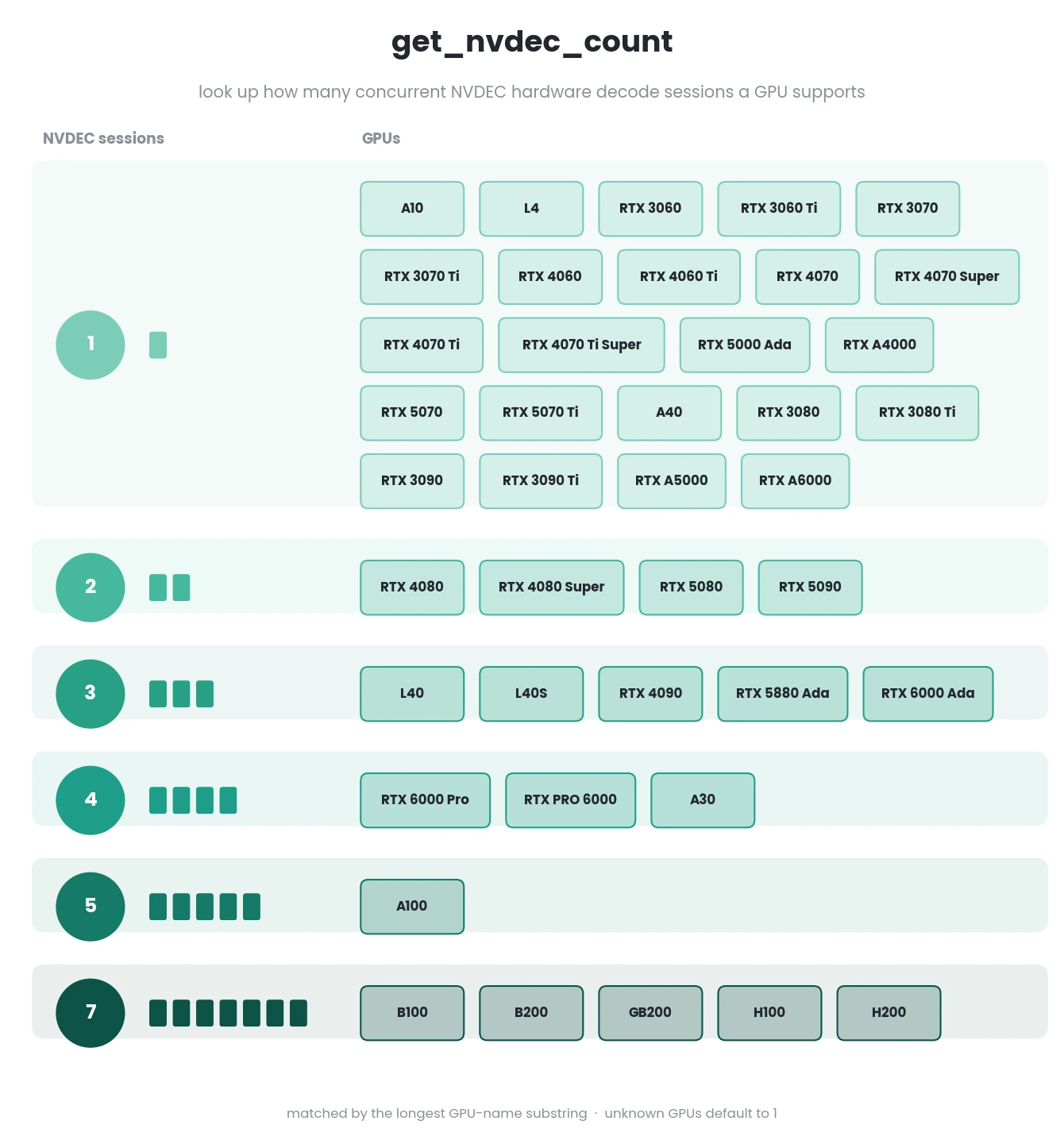
Note

When gpu_name is None, the first GPU name reported by nvidia-smi is used. Matching is done by substring: the longest dictionary key contained in gpu_name wins, so shorter names do not shadow longer ones (e.g. RTX 4070 Ti Super before RTX 4070 Ti). Unknown or unmatched GPUs return 1.

Parameters: gpu_name (str | None) – Full GPU product string, or None to query the local GPU.
Returns: NVDEC engine count used for capacity hints (defaults to 1 if unknown).
Return type: int

simba.utils.lookups.get_random_color_palette(n_colors: int)[source]: Get a random color palette with N random colors.

simba.utils.lookups.get_table(data: Dict[str, Any], headers: Optional[Tuple[str, str]] = ('SETTING', 'VALUE'), tablefmt: str = 'grid') → str[source]

Create a formatted table string from dictionary data using the tabulate library.

Converts a dictionary into a formatted table string suitable for display or printing. Each key-value pair in the dictionary becomes a row in the table.

Parameters

data (Dict[str, Any]) – Dictionary containing the data to be formatted as a table. Keys become the first column, values become the second column.
headers (Optional[Tuple[str, str]]) – Tuple of two strings representing the column headers. Default is (“SETTING”, “VALUE”).
tablefmt (Literal["grid"]) – Table format style. For options, see simba.utils.enums.Formats.VALID_TABLEFMT

Return str

Formatted table string ready for display or printing.

Example

>>> data = {"fps": 30, "width": 1920, "height": 1080, "frame_count": 3000}
>>> table = get_table(data=data, headers=("PARAMETER", "VALUE"))

simba.utils.lookups.get_third_party_appender_file_formats() → Dict[str, str][source]: Helper to get dictionary that maps different third-party annotation tools with different file formats.

simba.utils.lookups.get_tooltips() → Dict[str, str][source]

simba.utils.lookups.gpu_quality_to_cpu_quality_lk()[source]

simba.utils.lookups.integer_to_cardinality_lookup()[source]: Create dictionary that maps integers to cardinal compass directions.

simba.utils.lookups.intermittent_palette(n: int = 10, base_light: float = 0.55, contrast_delta: float = 0.18, seed_hue: Optional[float] = None, output: typing_extensions.Literal['rgb', 'rgb255', 'hex'] = 'rgb', rng: Optional[Random] = None) → Union[List[Tuple[float, float, float]], List[Tuple[int, int, int]], List[str]][source]

Generate a categorical colour palette with evenly spaced hues and alternating lightness.

Note

Use to get color palette where immediate colors are distinct.

Parameters

n (int) – Number of colours to generate. Must be greater than or equal to 1.
base_light (float) – Midpoint HSV value (0-1) used as the baseline lightness. Default 0.55.
contrast_delta (float) – Lightness offset added/subtracted per colour to improve visual separation. Default 0.18.
seed_hue (Optional[float]) – Initial hue (0-1). If None, a random hue is sampled. Default None.
output (str) – Output colour format. One of {"rgb", "rgb255", "hex"}. Default "rgb".
rng (Optional[random.Random]) – Optional pre-seeded RNG for reproducible random starts.

Returns

Colour palette in the requested format (RGB floats, RGB 0-255 integers, or hexadecimal strings).

Return type

Union[List[Tuple[float, float, float]], List[Tuple[int, int, int]], List[str]]

Example

>>> palette = intermittent_palette(n=6, output="hex")
>>> palette
>>> ['#a33f46', '#51a5df', '#b36824', '#4dbd9f', '#c749b4', '#7a9a3e']

simba.utils.lookups.is_running_in_ide()[source]

simba.utils.lookups.load_simba_fonts()[source]: Load fonts defined in simba.utils.enums.FontPaths into memory

simba.utils.lookups.percent_to_crf_lookup() → Dict[str, int][source]: Create dictionary that matches human-readable percent values to FFmpeg Constant Rate Factor (CRF) values that regulates video quality in CPU codecs. Higher CRF values translates to lower video quality and reduced file sizes.

simba.utils.lookups.percent_to_qv_lk()[source]: Create dictionary that matches human-readable percent values to FFmpeg regulates video quality in CPU codecs. Higher FFmpeg quality scores maps to smaller, lower quality videos. Used in some AVI codecs such as ‘divx’ and ‘mjpeg’.

simba.utils.lookups.print_video_meta_data(data_path: Union[str, PathLike]) → None[source]

Print video metadata as formatted tables to the console.

This function reads video metadata from either a single video file or all video files in a directory, then prints the metadata as formatted tables.

See also

To get video metadata as a dictionary without printing, use simba.utils.read_write.get_video_meta_data(). To get video metadata as a table without printing, use simba.utils.lookups.get_table().

Parameters: data_path (Union[str, os.PathLike]) – Path to video file or directory containing videos.
Returns: None. Video metadata is printed as formatted tables in the main console.

simba.utils.lookups.quality_pct_to_crf(pct: int) → int[source]

simba.utils.lookups.rgb_to_hex(color: Tuple[int, int, int]) → str[source]

simba.utils.lookups.video_quality_to_preset_lookup() → Dict[str, str][source]: Create dictionary that matches human-readable video quality settings to FFmpeg presets for GPU codecs.

simba.utils.lookups.win_to_wsl_path(win_path: Union[str, PathLike]) → str[source]: Helper to convert a windows path name, to a WSL path name

SimBA Printing

class simba.utils.printing.SimbaTimer(start: bool = False, perf_counter: bool = False)[source]

Bases: object

Timer class for keeping track of start and end-times of calls

start_timer()[source]

stop_timer()[source]

simba.utils.printing.log_event(logger_name: str, log_type: typing_extensions.Literal['CLASS_INIT', 'error', 'warning'], msg: str)[source]

simba.utils.printing.perform_timing(func)[source]

simba.utils.printing.stdout_information(msg: str, source: Optional[str] = '', elapsed_time: Optional[str] = None) → None[source]

Helper to parse information msg to SimBA main interface. E.g., how many monitors and their resolutions which is available.

Parameters

msg (str) – Message to be parsed.
source (Optional[str]) – Optional string indicating the source method or function of the operation for logging.
elapsed_time – Optional string indicating the runtime.

Return None

simba.utils.printing.stdout_success(msg: str, source: Optional[str] = '', elapsed_time: Optional[str] = None) → None[source]

Helper to parse msg of completed operation to SimBA main interface.

Parameters

msg (str) – Message to be parsed.
source (Optional[str]) – Optional string indicating the source method or function of the msg for logging.
elapsed_time (Optional[str]) – Optional string indicating the runtime of the completed operation.

Return None

simba.utils.printing.stdout_trash(msg: str, source: Optional[str] = '', elapsed_time: Optional[str] = None) → None[source]

Helper to parse msg of delete operation to SimBA main interface.

Parameters

msg (str) – Message to be parsed.
source (Optional[str]) – Optional string indicating the source method or function of the operation for logging.
elapsed_time – Optional string indicating the runtime.

Return None

simba.utils.printing.stdout_warning(msg: str, elapsed_time: Optional[str] = None) → None[source]

Helper to parse warning msg to SimBA main interface.

Parameters

msg (str) – Message to be parsed.
source (Optional[str]) – Optional string indicating the source method or function of the msg for logging.
elapsed_time – Optional string indicating the runtime.

Return None

Reading and writing

simba.utils.read_write.archive_processed_files(config_path: Union[str, PathLike], archive_name: str) → None[source]

Archive files within a SimBA project.

Parameters

config_path (str) – Path to SimBA project project_config.ini.
archive_name (str) – Name of archive.

See also

Tutorial

Example

>>> archive_processed_files(config_path='project_folder/project_config.ini', archive_name='my_archive')

simba.utils.read_write.bento_file_reader(file_path: Union[str, PathLike], fps: Optional[float] = None, orient: Optional[typing_extensions.Literal['index', 'columns']] = 'index', save_path: Optional[Union[str, PathLike]] = None, raise_error: Optional[bool] = False, log_setting: Optional[bool] = False) → Union[None, Dict[str, DataFrame]][source]

Reads a BENTO annotation file and processes it into a dictionary of DataFrames, each representing a classified behavior. Optionally, the results can be saved to a specified path.

The function handles both frame-based and second-based annotations, converting the latter to frame-based annotations if the frames-per-second (FPS) is provided or can be inferred from the file.

Parameters

file_path (Union[str, os.PathLike]) – Path to the BENTO annotation file.
fps (Optional[float]) – Frames per second (FPS) for converting second-based annotations to frames. If not provided, the function will attempt to infer FPS from the file. If FPS is required and cannot be inferred, an error is raised.
save_path (Optional[Union[str, os.PathLike]]) – Path to save the processed results as a pickle file. If None, results are returned instead of saved.

Returns

A dictionary where the keys are classifier names and the values are DataFrames with ‘START’ and ‘STOP’ columns representing the start and stop frames of each behavior.

Return type

Dict[str, pd.DataFrame]

Example

>>> bento_file_reader(file_path=r"C:/troubleshooting/bento_test/bento_files/20240812_crumpling3.annot")

simba.utils.read_write.bgr_to_rgb_tuple(value: Tuple[int, int, int]) → Tuple[int, int, int][source]: convert bgr tuple to rgb tuple

simba.utils.read_write.check_if_hhmmss_timestamp_is_valid_part_of_video(timestamp: str, video_path: Union[str, PathLike]) → None[source]

Helper to check that a timestamp in HH:MM:SS format is a valid timestamp in a video file.

Parameters

timestamp (str) – Timestamp in HH:MM:SS format.
video_path (str) – Path to a video file.

Raises

FrameRangeError – If timestamp is not in the video file. E.g., timestamp 00:01:00 will raise FrameRangeError if the video is 59s long.

Example

>>> check_if_hhmmss_timestamp_is_valid_part_of_video(timestamp='01:00:05', video_path='/Users/simon/Desktop/video_tests/Together_1.avi')
>>> "FrameRangeError: The timestamp '01:00:05' does not occur in video Together_1.avi, the video has length 10s"

simba.utils.read_write.clean_sleap_file_name(filename: str) → str[source]

Clean a SLEAP input filename by removing ‘.analysis’ suffix, the video number, and project name prefix, to match orginal video name.

Note

Modified from vtsai881.

Parameters: filename (str) – The original filename to be cleaned to match video name.
Returns str: The cleaned filename.
Example

>>> clean_sleap_file_name("projectname.v00x.00x_videoname.analysis.csv")
>>> 'videoname.csv'
>>> clean_sleap_file_name("projectname.v00x.00x_videoname.analysis.h5")
>>> 'videoname.h5'

simba.utils.read_write.clean_sleap_filenames_in_directory(dir: Union[str, PathLike], verbose: bool = False) → None[source]

Clean up SLEAP input filenames in the specified directory by removing a prefix and a suffix, and renaming the files to match the names of the original video files.

Note

Modified from vtsai881.

Parameters: dir (Union[str, os.PathLike]) – The directory path where the SLEAP CSV or H5 files are located.
Example

>>> clean_sleap_filenames_in_directory(dir='/Users/simon/Desktop/envs/troubleshooting/Hornet_SLEAP/import/')

simba.utils.read_write.clean_superanimal_topview_filename(file_name: str)[source]

simba.utils.read_write.concatenate_videos_in_folder(in_folder: Union[str, PathLike, bytes], save_path: Union[str, PathLike], file_paths: Optional[List[Union[str, PathLike]]] = None, video_format: Optional[str] = 'mp4', substring: Optional[str] = None, remove_splits: Optional[bool] = True, gpu: Optional[bool] = False, fps: Optional[Union[int, str]] = None, verbose: bool = True) → None[source]

Concatenate (temporally) all video files in a folder into a single video.

Important

Input video parts will be joined in alphanumeric order, should ideally have to have sequential numerical ordered file names, e.g., 1.mp4, 2.mp4….

Note

If substring and file_paths are both not None, then file_paths with be sliced and only file paths with substring will be retained.

Parameters

in_folder (Union[str, os.PathLike]) – Path to folder holding un-concatenated video files.
save_path (Union[str, os.PathLike]) – Path to the saved the output file. Note: If the path exist, it will be overwritten
file_paths (Optional[List[Union[str, os.PathLike]]]) – If not None, then the files that should be joined. If None, then all files. Default None.
video_format (Optional[str]) – The format of the video clips that should be concatenated. Default: mp4.
substring (Optional[str]) – If a string, then only videos in in_folder with a filename that contains substring will be joined. If None, then all are joined. Default: None.
video_format – Format of the input video files in in_folder. Default: mp4.
remove_splits (Optional[bool]) – If true, the input splits in the in_folder will be removed following concatenation. Default: True.

Return type

None

simba.utils.read_write.convert_csv_to_parquet(directory: Union[str, PathLike]) → None[source]

Convert all csv files in a folder to parquet format.

Parameters: directory (str) – Path to directory holding csv files.
Raises: NoFilesFoundError – The directory has no csv files.
Examples

>>> convert_parquet_to_csv(directory='project_folder/csv/input_csv')

simba.utils.read_write.convert_parquet_to_csv(directory: str) → None[source]

Convert all parquet files in a directory to csv format.

Parameters: directory (str) – Path to directory holding parquet files
Raises: NoFilesFoundError – The directory has no parquet files.
Examples

>>> convert_parquet_to_csv(directory='project_folder/csv/input_csv')

simba.utils.read_write.copy_files_in_directory(in_dir: Union[str, PathLike], out_dir: Union[str, PathLike], raise_error: bool = True, filetype: Optional[str] = None, prefix: Optional[str] = None, verbose: Optional[bool] = False, skip_truncated_img: Optional[bool] = False) → None[source]

Copy files from the specified input directory to the output directory.

Parameters

in_dir (Union[str, os.PathLike]) – The input directory from which files will be copied.
out_dir (Union[str, os.PathLike]) – The output directory where files will be copied to.
raise_error (bool) – If True, raise an error if no files are found in the input directory. Default is True.
filetype (Optional[str]) – If specified, only copy files with the given file extension. Default is None, meaning all files will be copied.
prefix (Optional[str]) – If specified, the given prefix will be added to the copied files’ names.

Example

>>> copy_files_in_directory('/input_dir', '/output_dir', raise_error=True, filetype='txt')

simba.utils.read_write.copy_files_to_directory(file_paths: Union[List[Union[str, PathLike]], str, PathLike], dir: Union[str, PathLike], verbose: Optional[bool] = True, overwrite: bool = True, check_validity: bool = True, integer_save_names: Optional[bool] = False) → List[Union[str, PathLike]][source]

Copy a list of files to a specified directory.

Parameters

file_paths (List[Union[str, os.PathLike]]) – List of paths to the files to be copied, or a single filepath string.
dir (Union[str, os.PathLike]) – Path to the directory where files will be copied.
verbose (Optional[bool]) – If True, prints progress information. Default True.
integer_save_names (Optional[bool]) – If True, saves files with integer names. E.g., file one in file_paths will be saved as dir/0.

Return List[Union[str, os.PathLike]]

List of paths to the copied files

simba.utils.read_write.copy_multiple_videos_to_project(config_path: Union[str, PathLike], source: Union[str, PathLike], file_type: str, symlink: Optional[bool] = False, recursive_search: Optional[bool] = False, allowed_video_formats: Optional[Tuple[str]] = ('avi', 'mp4')) → None[source]

Import directory of videos to SimBA project.

Parameters

config_path (Union[str, os.PathLike]) – path to SimBA project config file in Configparser format
source (Union[str, os.PathLike]) – Path to directory with video files outside SimBA project.
file_type (str) – Video format of imported videos (i.e.,: mp4 or avi)
symlink (Optional[bool]) – If True, creates soft copies rather than hard copies. Default: False.
recursive_search (Optional[bool]) – If True, copies all video files in subdirectories and immediately in source. If False, only files immediately in source. Default: False.
allowed_video_formats (Optional[Tuple[str]]) – Allowed video formats. DEFAULT: avi or mp4

simba.utils.read_write.copy_single_video_to_project(simba_ini_path: Union[str, PathLike], source_path: Union[str, PathLike], symlink: bool = False, allowed_video_formats: Optional[Tuple[str]] = ('avi', 'mp4'), overwrite: Optional[bool] = False) → None[source]

Import single video file to SimBA project

Parameters

simba_ini_path (Union[str, os.PathLike]) – path to SimBA project config file in Configparser format
source_path (Union[str, os.PathLike]) – Path to video file outside SimBA project.
symlink (Optional[bool]) – If True, creates soft copy rather than hard copy. Default: False.
allowed_video_formats (Optional[Tuple[str]]) – Allowed video formats. DEFAULT: avi or mp4
overwrite (Optional[bool]) – If True, overwrites existing video if it exists in SimBA project. Else, raise FileExistError.

simba.utils.read_write.create_directory(paths: Union[str, PathLike, bytes, List[str], Tuple[str]], overwrite: bool = False, verbose: bool = False) → None[source]

Create one or multiple directories.

Parameters

paths (Union[str, os.PathLike, bytes, List[str], Tuple[str]]) – A single path or a list/tuple of paths to create. Each path must be a non-empty string.
overwrite – If True and the directory already exists, it will be deleted and recreated. If False, the existing directory will be preserved.

Returns

None

simba.utils.read_write.create_empty_xlsx_file(xlsx_path: Union[str, PathLike])[source]: Create an empty MS Excel file. :param Union[str, os.PathLike] xlsx_path: Path where to save MS Excel file on disk.

simba.utils.read_write.df_to_xlsx_sheet(xlsx_path: Union[str, PathLike], df: DataFrame, sheet_name: str, create_file: bool = True) → None[source]

Append a DataFrame as a new worksheet in an Excel workbook.

If xlsx_path does not exist and create_file is True, an empty workbook is created first. The function then appends df as a new sheet. If a sheet with sheet_name already exists, a DuplicationError is raised.

Note

The DataFrame index is written to Excel because DataFrame.to_excel is called with default settings.

Parameters

xlsx_path (Union[str, os.PathLike]) – Path to the target .xlsx file.
df (pd.DataFrame) – DataFrame to write into the new worksheet.
sheet_name (str) – Name of the worksheet to create.
create_file (bool) – If True, create a new workbook when xlsx_path is missing. If False, raise NoFilesFoundError when the file does not exist.

Returns

None.

Return type

None

Raises

NoFilesFoundError – If xlsx_path does not exist and create_file is False.
DuplicationError – If sheet_name already exists in the workbook.
InvalidInputError – If inputs fail validation.

simba.utils.read_write.drop_df_fields(data: DataFrame, fields: List[str], raise_error: Optional[bool] = False) → DataFrame[source]

Drops specified fields in dataframe.

Parameters

pd.DataFrame – Data in pandas format.
fields (List[str]) – Columns to drop.

:return pd.DataFrame

simba.utils.read_write.extract_audio_from_video(video_path: Union[str, PathLike], save_path: Union[str, PathLike], bitrate: str = '192k', sample_rate: int = 44100) → None[source]

Extract audio track from video file and save as MP3.

Parameters

video_path (Union[str, os.PathLike]) – Path to input video file.
save_path (Union[str, os.PathLike]) – Path where the MP3 file will be saved.
bitrate (str) – Audio bitrate (e.g., ‘128k’, ‘192k’, ‘320k’). Default: ‘192k’.
sample_rate (int) – Audio sample rate in Hz. Default: 44100.

Raises

InvalidInputError – If video has no audio track or ffmpeg is not available.
FFMPEGCodecGPUError – If ffmpeg extraction fails.

Example

>>> extract_audio_from_video(video_path='my_video.mp4', save_path='audio.mp3')
>>> extract_audio_from_video(video_path='my_video.mp4', save_path='audio.mp3', bitrate='320k')

simba.utils.read_write.fetch_pip_data(pip_url: str = 'https://pypi.org/pypi/simba-uw-tf-dev/json', time_out: int = 2) → Union[Tuple[Dict[str, Any], str], Tuple[None, None]][source]

Fetch PyPI package metadata from a PyPI JSON API URL.

Retrieves package information from the PyPI JSON API endpoint and extracts the latest version. Used primarily for checking if newer versions of SimBA are available. Returns the full JSON response data and the latest version string, or (None, None) if the request fails.

Parameters: pip_url (str) – URL to the PyPI JSON API endpoint for the package. Defaults to SimBA’s PyPI URL.
Returns: Tuple containing (JSON data dictionary, latest version string) on success, or (None, None) on failure.
Return type: Union[Tuple[Dict[str, Any], str], Tuple[None, None]]
Example

>>> json_data, version = fetch_pip_data()
>>> if version:
>>>     print(f"Latest version: {version}")

simba.utils.read_write.find_all_videos_in_directory(directory: Union[str, PathLike], as_dict: bool = False, raise_error: bool = False, video_formats: Tuple[str] = ('.avi', '.mp4', '.mov', '.flv', '.m4v', '.webm'), sort_alphabetically: bool = False) → Union[dict, list][source]

Get all video file paths within a provided directory

Parameters

directory (str) – Directory to search for video files.
as_dict (bool) – If True, returns dictionary with the video name as key and file path as value.
raise_error (bool) – If True, raise error if no videos are found. Else, NoFileFoundWarning.
video_formats (Tuple[str]) – Acceptable video formats. Default: ‘.avi’, ‘.mp4’, ‘.mov’, ‘.flv’, ‘.m4v’.

:return Either a list or dictionary of all available video files in the directory. :rtype: Union[dict, list]

Raises: NoFilesFoundError – If raise_error and directory has no files in formats video_formats.
Examples

>>> find_all_videos_in_directory(directory='project_folder/videos')

simba.utils.read_write.find_all_videos_in_project(videos_dir: Union[str, PathLike], basename: Optional[bool] = False, raise_error: bool = True) → List[str][source]

Get filenames of .avi and .mp4 files within a directory

Parameters

videos_dir (str) – Directory holding video files.
basename (bool) – If true returns basenames, else file paths.

Example

>>> find_all_videos_in_project(videos_dir='project_folder/videos')
>>> ['project_folder/videos/Together_2.avi', 'project_folder/videos/Together_3.avi', 'project_folder/videos/Together_1.avi']

simba.utils.read_write.find_closest_readable_frame(video_path: Union[str, PathLike], target_frame: int, max_search_range: int = 50) → Tuple[Optional[ndarray], Optional[int]][source]

Finds the closest readable frame to a target frame index.

This function attempts to read the target frame from a video. If the target frame cannot be read (e.g., due to corruption or encoding issues), it searches nearby frames in both directions to find the closest readable frame.

Parameters

video_path (Union[str, os.PathLike]) – Path to video file.
target_frame (int) – Target frame index to read (0-based).
max_search_range (int) – Maximum number of frames to search in each direction from target. Default: 100.

Returns

Tuple of (frame array, actual frame index) or (None, None) if no readable frame found.

Return type

Tuple[Optional[np.ndarray], Optional[int]]

Example

>>> frame, actual_idx = find_closest_readable_frame(video_path='video.mp4', target_frame=10810)
>>> if frame is not None:
>>>     print(f"Read frame {actual_idx} (target was 10810, offset: {actual_idx - 10810})")

simba.utils.read_write.find_core_cnt() → Tuple[int, int][source]

Find the local cpu count and quarter of the cpu counts.

Return int: The local cpu count
Return int: The local cpu count // 4
Example

>>> find_core_cnt()
>>> (8, 2)

simba.utils.read_write.find_files_of_filetypes_in_directory(directory: Union[str, PathLike], extensions: Union[List[str], Tuple[str], str], raise_warning: bool = True, as_dict: bool = False, raise_error: bool = False, sort_alphabetically: bool = False) → Union[List[str], Dict[str, str]][source]

Find all files in a directory of specified extensions/types.

Parameters

directory (str) – Directory holding files.
extensions (List[str]) – Accepted file extensions as a list of string, string, or tuple.
raise_warning (bool) – If True, raise warning if no files are found. Default True.
raise_error (bool) – If True, raise error if no files are found. Default False.
as_dict (bool) – If True, returns a dictionary with all filenames as keys and filepaths as values. If False, then a list of all filepaths. Default False.

Returns

All files in directory with the specified extension(s).

Return type

Union[List[str], Dict[str, str]]

Example

>>> find_files_of_filetypes_in_directory(directory='project_folder/videos', extensions=['mp4', 'avi', 'png'], raise_warning=False)

simba.utils.read_write.find_largest_blob_location(imgs: Dict[int, ndarray], verbose: bool = False, video_name: Optional[str] = None, inclusion_zone: Optional[Union[Polygon, MultiPolygon]] = None) → Dict[int, ndarray][source]

Helper to find the largest connected component in binary image. E.g., Use to find a “blob” (i.e., animal) within a background subtracted image.

Parameters

imgs (Dict[int, np.ndarray]) – Dictionary of images where the key is the frame id and the value is an image in np.ndarray format.
verbose (bool) – If True, prints progress. Default: False.
video_name (video_name) – The name of the video being processed for interpretable progress msg if verbose.
inclusion_zones (Optional[np.ndarray]) – If not None, then 2D numpy array of ROI / shape vertices. If not None, the largest blob will be searched for only in the ROI.

Returns

Dictionary where the key is the frame id and the value is a 2D array with x and y coordinates.

Return type

Dict[int, np.ndarray]

simba.utils.read_write.find_max_vertices_coordinates(shapes: List[Union[Polygon, LineString, MultiPolygon, Point]], buffer: Optional[int] = None) → Tuple[int, int][source]

Find the maximum x and y coordinates among the vertices of a list of geometries.

Can be useful for plotting puposes, to dtermine the rquired size of the canvas to fit all geometries.

Parameters

shapes (List[Union[Polygon, LineString, MultiPolygon, Point]]) – A list of Shapely geometries including Polygons, LineStrings, MultiPolygons, and Points.
buffer (Optional[int]) – If int, adds to maximum x and y.

Returns

A two-part tuple containing the maximum x and y coordinates found among the vertices.

Return type

Tuple[int, int]

Example

>>> polygon = Polygon([(0, 0), (1, 0), (1, 1), (0, 1)])
>>> line = LineString([(1, 1), (2, 2), (3, 1), (4, 0)])
>>> multi_polygon = MultiPolygon([Polygon([(0, 0), (1, 0), (1, 1), (0, 1)]), Polygon([(1, 1), (2, 1), (2, 2), (1, 2)])])
>>> point = Point(3, 4)
>>> find_max_vertices_coordinates([polygon, line, multi_polygon, point])
>>> (4, 4)

simba.utils.read_write.find_time_stamp_from_frame_numbers(start_frame: int, end_frame: int, fps: float) → List[str][source]

Given start and end frame numbers and frames per second (fps), return a list of formatted time stamps corresponding to the frame range start and end time.

Parameters

start_frame (int) – The starting frame index.
end_frame (int) – The ending frame index.
fps (float) – Frames per second.

Returns

A list of time stamps in the format ‘HH:MM:SS:MS’.

Return type

List[str]

Example

>>> find_time_stamp_from_frame_numbers(start_frame=11, end_frame=20, fps=3.4)
>>> ['00:00:03:235', '00:00:05:882']

simba.utils.read_write.find_video_of_file(video_dir: Union[str, PathLike], filename: str, raise_error: Optional[bool] = False, warning: Optional[bool] = True, recursive: bool = False) → Optional[Union[str, PathLike]][source]

Helper to find the video file with the SimBA project that represents a known data file path.

Parameters

video_dir (str) – Directory holding putative video file.
filename (str) – Data file name (stem only, e.g. Video_1). Path separators are stripped to the basename.
raise_error (Optional[bool]) – If True, raise error if no file can be found. If False, returns None if no file can be found. Default: False
warning (Optional[bool]) – If True, print warning if no file can be found. If False, no warning is printed if file cannot be found. Default: False
recursive (bool) – If True, search subdirectories of video_dir for the video file. If False, only the top-level of video_dir is searched. Default: False. If several files are found as a match, the first one is returned.

Returns

Video file path, or None if not found.

Return type

Union[str, os.PathLike, None]

Examples

>>> find_video_of_file(video_dir='project_folder/videos', filename='Together_1')
>>> 'project_folder/videos/Together_1.avi'

simba.utils.read_write.get_all_clf_names(config: ConfigParser, target_cnt: int) → List[str][source]

Get all classifier names in a SimBA project.

Parameters

config (configparser.ConfigParser) – Parsed SimBA project_config.ini
target_cnt (int) – Count of models in SimBA project

Returns

Classifier model names

Return type

List[str]

Example

>>> get_all_clf_names(config=config, target_cnt=2)
>>> ['Attack', 'Sniffing']

simba.utils.read_write.get_audio_duration(audio_path: Union[str, PathLike]) → float[source]

Get duration of audio file in seconds using ffprobe.

Parameters: audio_path (Union[str, os.PathLike]) – Path to audio file.
Return float: Duration in seconds.

simba.utils.read_write.get_bp_headers(body_parts_lst: List[str]) → list[source]

Helper to create ordered list of all column header fields from body-part names for SimBA project dataframes.

Parameters: body_parts_lst (List[str]) – Body-part names in the SimBA prject
Returns: Body-part headers
Return type: List[str]
Examaple

>>> get_bp_headers(body_parts_lst=['Nose'])
>>> ['Nose_x', 'Nose_y', 'Nose_p']

simba.utils.read_write.get_cpu_pool(core_cnt: int = -1, maxtasksperchild: int = 8000, context: Optional[typing_extensions.Literal['fork', 'spawn', 'forkserver']] = None, verbose: bool = True, source: Optional[str] = None) → Pool[source]

Creates and returns a multiprocessing.Pool instance with platform-appropriate defaults and validation.

Parameters

core_cnt (int) – Number of worker processes. -1 uses all available cores. Default: -1.
maxtasksperchild (int) – Maximum number of tasks a worker process can complete before being replaced. Default: From Defaults.MAXIMUM_MAX_TASK_PER_CHILD.
context (Optional[Literal['fork', 'spawn', 'forkserver']]) – Multiprocessing start method. None uses platform default. Default: None.
verbose (bool) – If True, prints pool creation message with timestamp. Default: True.
source (Optional[str]) – Optional identifier string for logging purposes (e.g., ‘VideoProcessor’). Default: None.

Returns

Configured multiprocessing.Pool instance.

Return type

multiprocessing.Pool

Example

>>> pool = get_cpu_pool(core_cnt=4, source='FeatureExtractor')
>>> pool = get_cpu_pool(core_cnt=-1, context='spawn', verbose=True)
>>> pool = get_cpu_pool(core_cnt=8, maxtasksperchild=100, source='VideoProcessor')

simba.utils.read_write.get_current_time()[source]

simba.utils.read_write.get_desktop_path(raise_error: bool = False)[source]: Get the path to the user desktop directory

simba.utils.read_write.get_downloads_path(raise_error: bool = False)[source]: Get the path to the user downloads directory

simba.utils.read_write.get_env_pose_config_dir(raise_error: Optional[bool] = True)[source]: Locate and validate the pose_configurations directory in the active SimBA installation.

simba.utils.read_write.get_file_name_info_in_directory(directory: Union[str, PathLike], file_type: str) → Dict[str, str][source]

Get dict of all file paths in a directory with specified extension as values and file base names as keys.

Parameters

directory (str) – Directory containing files.
file_type (str) – File-type in directory of interest

Return dict

All found files as values and file base names as keys.

Example

>>> get_file_name_info_in_directory(directory='C:/project_folder/csv/machine_results', file_type='csv')
>>> {'Video_1': 'C:/project_folder/csv/machine_results/Video_1'}

simba.utils.read_write.get_fn_ext(filepath: Union[PathLike, str], raise_error: bool = True) → Union[Tuple[str, str, str], Tuple[None, None, None]][source]

Split file path into three components: (i) directory, (ii) file name, and (iii) file extension.

Parameters

filepath (Union[os.PathLike, str]) – Path to file.
raise_error (bool) – If True, raises InvalidFilepathError for invalid paths. If False, returns (None, None, None) for invalid paths. Default: True.

Returns

3-part tuple with file directory name, file name (w/o extension), and file extension. Returns (None, None, None) if invalid path and raise_error=False.

Return type

Union[Tuple[str, str, str], Tuple[None, None, None]]

Example

>>> get_fn_ext(filepath='C:/My_videos/MyVideo.mp4')
('C:/My_videos', 'MyVideo', '.mp4')
>>> get_fn_ext(filepath='invalid_path', raise_error=False)
(None, None, None)

simba.utils.read_write.get_h5_frame_count(path: Union[str, PathLike]) → Optional[int][source]

Return the number of frames (rows) in a DLC H5 file without loading the full data.

Inspects the H5 file’s structural metadata to read the row dimension cheaply, handling both common pandas-on-HDF storage modes:

format='table' (legacy DLC TF backend) → <key>/table shape[0].
format='fixed' (modern DLC PyTorch backend) → <key>/axis1 shape[0] or <key>/block0_values shape[0].

If the structural shortcut fails for any reason, falls back to a full pandas.read_hdf() read.

Parameters: path (Union[str, os.PathLike]) – Path to a DLC H5 file.
Returns: Number of frames in the file, or None if no row count could be determined.
Return type: Optional[int]
Example

>>> n = get_h5_frame_count(r'video_DLC_HrnetW32_..._el.h5')
>>> # 5400

simba.utils.read_write.get_memory_usage_array(x: ndarray) → Dict[str, float][source]

Calculates the memory usage of a NumPy array in bytes, megabytes, and gigabytes.

Parameters: x – A NumPy array for which memory usage will be calculated. It should be a valid NumPy array with a defined size and dtype.
Returns: A dictionary with memory usage information, containing the following keys: - “bytes”: Memory usage in bytes. - “megabytes”: Memory usage in megabytes. - “gigabytes”: Memory usage in gigabytes.

simba.utils.read_write.get_memory_usage_of_df(df: DataFrame) → Dict[str, float][source]

Get the RAM memory usage of a dataframe.

Parameters: df (pd.DataFrame) – Parsed dataframe
Returns: Dict holding the memory usage of the dataframe in bytes, mb, and gb.
Return type: Dict[str, float]
Example

>>> df = pd.DataFrame(np.random.randint(0,100,size=(100, 4)), columns=list('ABCD'))
>>> {'bytes': 3328, 'megabytes': 0.003328, 'gigabytes': 3e-06}

simba.utils.read_write.get_number_of_header_columns_in_df(df: DataFrame) → int[source]

Returns the count of non-numerical header rows in dataframe. E.g., can be helpful to determine if dataframe is multi-index columns.

Parameters: df (pd.DataFrame) – Dataframe to check the count of non-numerical header rows for.
Example

>>> get_number_of_header_columns_in_df(df='project_folder/csv/input_csv/Video_1.csv')
>>> 3

simba.utils.read_write.get_pkg_version(pkg: str, raise_error: Optional[bool] = False)[source]

Helper to get the version of a package in the current python environment.

Example

>>> get_pkg_version(pkg='simba-uw-tf-dev')
>>> 1.82.7
>>> get_pkg_version(pkg='bla-bla')
>>> None

simba.utils.read_write.get_recent_projects_paths(max: int = 15, sort_alphabetically: bool = True) → List[str][source]

simba.utils.read_write.get_site_packages_path(raise_error: Optional[bool] = True) → Union[None, PathLike, str][source]: Retrieve the path to the current Python environment’s site-packages directory.

simba.utils.read_write.get_unique_values_in_iterable(data: Iterable, name: Optional[str] = '', min: Optional[int] = 1, max: Optional[int] = None) → int[source]

Helper to get and check the number of unique variables in iterable. E.g., check the number of unique identified clusters.

Parameters

data (np.ndarray) – 1D iterable.
name (Optional[str]) – Arbitrary name of iterable for informative error messaging.
min (Optional[int]) – Optional minimum number of unique variables. Default 1.
max (Optional[int]) – Optional maximum number of unique variables. Default None.

simba.utils.read_write.get_video_info_ffmpeg(video_path: Union[str, PathLike]) → Dict[str, Any][source]

Extracts metadata information from a video file using FFmpeg’s ffprobe.

Note

FFMpeg based metadata extraction seems preferable over OpenCV with data in .h264 format.

See also

To use OpenCV instead of FFmpeg, see simba.utils.read_write.get_video_meta_data()

Parameters: video_path (Union[str, os.PathLike]) – The file path to the video for which metadata is to be extracted.
Returns: A dictionary containing video metadata:
Return type: Dict[str, Any]

simba.utils.read_write.get_video_meta_data(video_path: Union[str, PathLike, VideoCapture], fps_as_int: bool = True, raise_error: bool = True) → Optional[Dict[str, Any]][source]

Read video metadata (fps, resolution, frame cnt etc.) from video file (e.g., mp4).

See also

To use FFmpeg instead of OpenCV, see simba.utils.read_write.get_video_info_ffmpeg().

Parameters

video_path (str) – Path to a video file.
fps_as_int (bool) – If True, force video fps to int through floor rounding, else float. Default = True.
raise_error (bool) – If True, raises an error if data cannot be read. If False, returns None. Default True.

Returns

The video metadata in dict format with parameter (e.g., fps) as keys.

Return type

Dict[str, Any].

Example

>>> get_video_meta_data('test_data/video_tests/Video_1.avi')
{'video_name': 'Video_1', 'fps': 30, 'width': 400, 'height': 600, 'frame_count': 300, 'resolution_str': '400 x 600', 'video_length_s': 10}

simba.utils.read_write.img_array_to_clahe(img: ndarray, clip_limit: int = 2, tile_grid_size: Tuple[int, int] = (16, 16)) → ndarray[source]

simba.utils.read_write.img_stack_to_bw(imgs: ndarray)[source]

Jitted conversion of a 4D stack of color images (RGB format) to black and white.

Parameters: imgs (np.ndarray) – A 4D array representing color images. It should have the shape (num_images, height, width, 3) where the last dimension represents the color channels (R, G, B).
Returns np.ndarray: A 3D array containing the black and white versions of the input images. The shape of the output array is (num_images, height, width).
Example

>>> imgs = ImageMixin().read_img_batch_from_video( video_path='/Users/simon/Desktop/envs/troubleshooting/two_black_animals_14bp/videos/Together_1.avi', start_frm=0, end_frm=100)
>>> imgs = np.stack(list(imgs.values()))
>>> imgs_gray = ImageMixin.img_stack_to_greyscale(imgs=imgs)

simba.utils.read_write.img_stack_to_greyscale(imgs: ndarray)[source]

Jitted conversion of a 4D stack of color images (RGB format) to grayscale.

Parameters: imgs (np.ndarray) – A 4D array representing color images. It should have the shape (num_images, height, width, 3) where the last dimension represents the color channels (R, G, B).
Returns np.ndarray: A 3D array containing the grayscale versions of the input images. The shape of the output array is (num_images, height, width).
Example

>>> imgs = ImageMixin().read_img_batch_from_video( video_path='/Users/simon/Desktop/envs/troubleshooting/two_black_animals_14bp/videos/Together_1.avi', start_frm=0, end_frm=100)
>>> imgs = np.stack(list(imgs.values()))
>>> imgs_gray = ImageMixin.img_stack_to_greyscale(imgs=imgs)

simba.utils.read_write.img_stack_to_video(x: ndarray, save_path: Union[str, PathLike], fps: float, gpu: Optional[bool] = False, bitrate: Optional[int] = 5000) → None[source]

Converts a NumPy image stack to a video file, with optional GPU acceleration and configurable bitrate.

Parameters

x (np.ndarray) – A NumPy array representing the image stack. The array should have shape (N, H, W) for greyscale or (N, H, W, 3) for RGB images, where N is the number of frames, H is the height, and W is the width.
save_path (Union[str, os.PathLike]) – Path to the output video file where the video will be saved.
fps (float) – Frames per second for the output video. Should be a positive floating-point number.
gpu (Optional[bool]) – Whether to use GPU acceleration for encoding. If True, the video encoding will use NVIDIA’s NVENC encoder. Defaults to False.
bitrate (Optional[int]) – Bitrate for the video encoding in kilobits per second (kbps). Should be an integer between 1000 and 35000. Defaults to 5000.

Returns

None

simba.utils.read_write.img_to_bw(img: ndarray) → ndarray[source]

Jitted conversion of a single image (grayscale or RGB) to black and white.

Parameters: img – A 2D grayscale image (H, W) or 3D RGB image (H, W, 3), dtype uint8.
Returns: A 2D binary black and white image with values 0 or 255.

simba.utils.read_write.labelme_to_dlc(labelme_dir: Union[str, PathLike], scorer: Optional[str] = 'SN', save_dir: Optional[Union[str, PathLike]] = None) → None[source]

Convert labels from labelme format to DLC format.

Parameters

labelme_dir (Union[str, os.PathLike]) – Directory with labelme json files.
scorer (Optional[str]) – Name of the scorer (anticipated by DLC as header)
save_dir (Optional[Union[str, os.PathLike]]) – Directory where to save the DLC annotations. If None, then same directory as labelme_dir with _dlc_annotations suffix.

Returns

None

Example

>>> labelme_dir = r'D:/ts_annotations'
>>> labelme_to_dlc(labelme_dir=labelme_dir)

simba.utils.read_write.osf_download(project_id: str, save_dir: Union[str, PathLike], storage: str = 'osfstorage', overwrite: bool = False)[source]

Download all files from an OSF (Open Science Framework) project to a local directory.

This function connects to the OSF API, accesses the specified project and storage location, and downloads all files to the local save directory. Files can be skipped if they already exist locally and overwrite is disabled.

Parameters

project_id (str) – OSF project identifier (e.g., ‘abc123’ from osf.io/abc123).
save_dir (Union[str, os.PathLike]) – Local directory path where files will be downloaded.
storage (str) – OSF storage location name (default: ‘osfstorage’).
overwrite (bool) – If True, overwrite existing files. If False, skip existing files (default: False).

Example

>>> osf_download(project_id="7fgwn", save_dir=r'E:/rgb_white_vs_black_imgs')
>>> osf_download(project_id="kym42", save_dir=r'E:/crim13_imgs', overwrite=True)

simba.utils.read_write.read_boris_file(file_path: Union[str, PathLike], fps: Optional[Union[float, int]] = None, orient: Optional[typing_extensions.Literal['index', 'columns']] = 'index', save_path: Optional[Union[str, PathLike]] = None, raise_error: Optional[bool] = False, log_setting: Optional[bool] = False) → Union[None, Dict[str, Dict[str, DataFrame]]][source]

Reads a BORIS behavioral annotation file, processes the data, and optionally saves the results to a file.

Parameters

file_path (Union[str, os.PathLike]) – The path to the BORIS file to be read. The file should be a CSV containing behavioral annotations.
fps (Optional[Union[int, float]]) – Frames per second (FPS) to convert time annotations into frame numbers. If not provided, it will be extracted from the BORIS file if available.
orient (Optional[Literal['index', 'columns']]) – Determines the orientation of the results. ‘index’ will organize data with start and stop times as indices, while ‘columns’ will store data in columns.
save_path (Optional[Union[str, os.PathLike]) – The path where the processed results should be saved as a pickle file. If not provided, the results will be returned instead.
raise_error (Optional[bool]) – Whether to raise errors if the file format or content is invalid. If False, warnings will be logged instead of raising exceptions.
log_setting (Optional[bool]) – Whether to log warnings and errors. This is relevant when raise_error is set to False.

Returns

If save_path is None, returns a dictionary where keys are behaviors and values are dataframes containing start and stop frames for each behavior. If save_path is provided, the results are saved and nothing is returned.

simba.utils.read_write.read_config_entry(config: ConfigParser, section: str, option: str, data_type: str, default_value: Optional[Any] = None, options: Optional[List] = None) → Union[float, int, str][source]

Helper to read entry in SimBA project_config.ini parsed by configparser.ConfigParser.

Parameters

config (configparser.ConfigParser) – Parsed SimBA project_config.ini. Use simba.utils.read_config_file() to parse file.
section (str) – Section name of entry to parse.
option (str) – Option name of entry to parse.
data_type (str) – Type of data to parse. E.g., str, int, float.
default_value (Optional[Any]) – If no matching entry can be found in the project_config.ini, use this as default.
options (Optional[List] or None) – List of valid options. If not None, checks that the returned entry value exists in this list.

:return Any

Example

>>> read_config_entry(config='project_folder/project_config.ini', section='General settings', option='project_name', data_type='str')
>>> 'two_animals_14_bps'

simba.utils.read_write.read_config_file(config_path: Union[str, PathLike]) → ConfigParser[source]

Helper to parse SimBA project project_config.ini file

Parameters: config_path (Union[str, os.PathLike]) – Path to project_config.ini file
Returns: parsed project_config.ini file
Return type: configparser.ConfigParser
Raises: MissingProjectConfigEntryError – Invalid file format.
Example

>>> read_config_file(config_path='project_folder/project_config.ini')

simba.utils.read_write.read_data_paths(path: Optional[Union[str, PathLike]], default: List[Union[str, PathLike]], default_name: Optional[str] = '', file_type: Optional[str] = 'csv') → List[str][source]

Helper to flexibly read in a set of file-paths.

Parameters

path (Union[str, os.PathLike]) – None or path to a file or a folder or list of paths to files.
default (List[Union[str, os.PathLike]]) – If path is None. Use this passed list of file paths.
default_name (Optional[str]) – A readable name representing the default for interpretable error msgs. Defaults to empty string.
file_type (Optional[str]) – If path is a directory, read in all files in directory with this file extension. Default: csv.

Return List[str]

List of file paths.

simba.utils.read_write.read_df(file_path: Union[str, PathLike], file_type: Union[str, PathLike] = 'csv', has_index: Optional[bool] = True, remove_columns: Optional[List[str]] = None, usecols: Optional[List[str]] = None, anipose_data: Optional[bool] = False, check_multiindex: Optional[bool] = False, multi_index_headers_to_keep: Optional[int] = None, verbose: Optional[bool] = False) → Union[DataFrame, dict][source]

Read single tabular data file or pickle

Note

For improved runtime, defaults to pyarrow.csv.write_cs() if file type is csv.

EXPECTED RUNTIMES
CSV DISK SIZE (MB)	TIME (S)	STDEV TIME (S)
257	0.682866667	0.063618891
643	1.551066667	0.048732057
6435	22.01703333	0.612539014
7722	39.37053333	8.153716055

Parameters

file_path (str) – Path to data file
file_type (str) – Type of data. OPTIONS: ‘parquet’, ‘csv’, ‘pickle’.
Optional[bool] – If the input file has an initial index column. Default: True.
remove_columns (Optional[List[str]]) – If not None, then remove columns in lits.
usecols (Optional[List[str]]) – If not None, then keep columns in list.
check_multiindex (bool) – check file is multi-index headers. Default: False.
multi_index_headers_to_keep (int) – If reading multi-index file, and we want to keep one of the dropped multi-index levels as the header in the output file, specify the index of the multiindex hader as int.

Returns

Table data in pd.DataFrame format.

Return type

pd.DataFrame

Example

>>> read_df(file_path='project_folder/csv/input_csv/Video_1.csv', file_type='csv', check_multiindex=True)

simba.utils.read_write.read_df_array(df: DataFrame, column: str)[source]

Convert string representations of 2D arrays in a DataFrame column to actual numpy arrays.

Parameters

df (pd.DataFrame) – The DataFrame containing the column.
column (str) – The name of the column with string representations of 2D arrays.

Returns

A list of numpy arrays, each corresponding to an entry in the specified column.

Return type

List[np.ndarray]

simba.utils.read_write.read_dlc_superanimal_h5(path: Union[str, PathLike], col_names: List[str]) → DataFrame[source]

Read and parse DeepLabCut SuperAnimal-TopView pose estimation data from H5 format.

Supports both DLC H5 layouts that the SuperAnimal-TopView workflow can produce:

Legacy DLC TensorFlow backend — H5 contains a df_with_missing group with a nested PyTables table (DLC <= 2.x export written with df.to_hdf(..., key='df_with_missing', format='table')).
Modern DLC 3.0+ PyTorch backend (HRNet / RTMPose, including multi-animal _el.h5 / _full.h5 outputs) — H5 stores a pandas DataFrame with a multi-index column header (typical levels: scorer / [individuals] / bodyparts / coords). Readable directly with pandas.read_hdf().

Regardless of the source format, the returned DataFrame has its columns assigned to col_names positionally. The H5 column order is therefore assumed to follow the SimBA project’s body-part order (i.e. SuperAnimal-TopView 27 body parts per animal, each as an x, y, likelihood triplet, animals in the order specified by id_lst in simba.pose_importers.superanimal_import.SuperAnimalTopViewImporter).

Parameters

path (Union[str, os.PathLike]) – Path to the SuperAnimal DLC H5 file.
col_names (List[str]) – List of column names to assign to the DataFrame. Must match the expected number of columns based on the SimBA project configuration (typically body-part coordinates: x, y, p).

Returns

DataFrame containing pose estimation data with columns named according to col_names.

Return type

pd.DataFrame

Raises

InvalidInputError – If the file cannot be read by any supported strategy, or if the number of columns in the file is less than the number of expected column names.

Example

>>> col_names = ['Animal_1_Nose_x', 'Animal_1_Nose_y', 'Animal_1_Nose_p', 'Animal_1_Ear_left_x', ...]
>>> df = read_dlc_superanimal_h5(path='project_folder/videos/Video_1.h5', col_names=col_names)

simba.utils.read_write.read_facemap_h5(file_path: Union[str, PathLike]) → DataFrame[source]

Convert FaceMap pose-estimation data to pandas Dataframe format.

See also

See FaceMap GitHub repository for expected H5 file format: https://github.com/MouseLand/facemap

Parameters: file_path (Union[str, os.PathLike]) – Path to facemap data file in .h5 format.
Returns: FaceMap pose-estimation data in DataFrame format.
Return type: pd.DataFrame

simba.utils.read_write.read_frm_of_video(video_path: Union[str, PathLike, VideoCapture], frame_index: Optional[int] = 0, opacity: Optional[float] = None, size: Optional[Tuple[int, int]] = None, keep_aspect_ratio: bool = False, greyscale: Optional[bool] = False, black_and_white: Optional[bool] = False, clahe: Optional[Union[Tuple[int, int, int], bool]] = False, use_ffmpeg: Optional[bool] = False, raise_error: Optional[bool] = True) → Optional[ndarray][source]

Reads a single frame from a video file.

See also

To read a batch of images with GPU acceleration, see simba.utils.read_write.read_img_batch_from_video_gpu(). To read a batch of videos using multicore CPU acceleration, see simba.utils.read_write.read_img_batch_from_video(). To read frames batches asynchronously, see simba.video_processors.async_frame_reader.AsyncVideoFrameReader().

Parameters

video_path (Union[str, os.PathLike, cv2.VideoCapture]) – Path to video file, or cv2.VideoCapture object.
frame_index (Optional[int]) – The frame index to return (0-based). Default: 0. If -1 is passed, the last frame of the video is read.
opacity (Optional[float]) – Value between 0 and 100 or None. If float value, returns image with opacity. 100 fully opaque. 0.0 fully transparent.
size (Optional[Tuple[int, int]]) – If tuple (width, height), resizes the image. If None, returns original image size. When used with keep_aspect_ratio=True, the image is resized to fit within the target size while maintaining aspect ratio.
keep_aspect_ratio (bool) – If True and size is provided, resizes the image to fit within the target size while maintaining aspect ratio. If False, resizes to exact size (may distort aspect ratio). Default False.
greyscale (Optional[bool]) – If True, returns the greyscale image. Default False.
black_and_white (Optional[bool]) – If True, returns black and white image at threshold 127. Default False.
clahe (Optional[Union[Tuple[int, int, int], bool]]) – CLAHE settings. If True, uses default CLAHE (clipLimit=2, tileGridSize=(16, 16)). If a 3-tuple, interpreted as (clip_limit, tile_x, tile_y). If False/None, CLAHE is not applied.
use_ffmpeg (Optional[bool]) – If True, uses FFmpeg for frame extraction instead of OpenCV. Default False.
raise_error (Optional[bool]) – If True, raises error on failure. If False, returns None on failure. Default True.

Returns

Image as numpy array, or None if raise_error=False and an error occurs.

Return type

Union[np.ndarray, None]

Example

>>> img = read_frm_of_video(video_path='/Users/simon/Desktop/envs/platea_featurizer/data/video/3D_Mouse_5-choice_MouseTouchBasic_s9_a4_grayscale.mp4')
>>> cv2.imshow('img', img)
>>> cv2.waitKey(5000)

simba.utils.read_write.read_img(img_path: Union[str, PathLike], greyscale: bool = False, clahe: bool = False, opacity: Optional[float] = None) → ndarray[source]

simba.utils.read_write.read_img_batch_from_video(video_path: Union[str, PathLike], start_frm: Optional[int] = None, end_frm: Optional[int] = None, greyscale: bool = False, black_and_white: bool = False, clahe: bool = False, core_cnt: int = -1, size: Optional[Tuple[int, int]] = None, pool: Optional[Pool] = None, verbose: bool = False) → Dict[int, ndarray][source]

Read a batch of frames from a video file. This method reads frames from a specified range of frames within a video file using multiprocessing.

EXPECTED RUNTIMES
READ FRAME COUNT	TIME (S)	STDEV (S)
1000	7.149766667	1.001209181
2000	8.874533333	0.258467219
REPEATS = 3
RESOLUTION: 670 x 530
CORES: 24

See also

For GPU acceleration, see simba.utils.read_write.read_img_batch_from_video_gpu()

Note

When black-and-white videos are saved as MP4, there can be some small errors in pixel values during compression. A video with only (0, 255) pixel values therefore gets other pixel values, around 0 and 255, when read in again. If you expect that the video you are reading in is black and white, set black_and_white to True to round any of these wonly value sto 0 and 255.

Parameters

video_path (Union[str, os.PathLike]) – Path to the video file.
start_frm (int) – Starting frame index.
end_frm (int) – Ending frame index.
core_cnt (Optionalint]) – Number of CPU cores to use for parallel processing. Default is -1, indicating using all available cores.
greyscale (Optional[bool]) – If True, reads the images as greyscale. If False, then as original color scale. Default: False.
black_and_white (bool) – If True, returns the images in black and white. Default False.
clahe (bool) – If True, returns clahe enhanced images.

Returns

A dictionary containing frame indices as keys and corresponding frame arrays as values.

Return type

Dict[int, np.ndarray]

Example

>>> read_img_batch_from_video(video_path='/Users/simon/Desktop/envs/troubleshooting/two_black_animals_14bp/videos/Together_1.avi', start_frm=0, end_frm=50)

simba.utils.read_write.read_img_batch_from_video_gpu(video_path: Union[str, PathLike], start_frm: Optional[int] = None, end_frm: Optional[int] = None, verbose: bool = False, greyscale: bool = False, black_and_white: bool = False, out_format: typing_extensions.Literal['dict', 'array'] = 'dict') → Union[Dict[int, ndarray], ndarray][source]

Reads a batch of frames from a video file using GPU acceleration.

EXPECTED RUNTIMES
READ FRAME COUNT	TIME (S)	STDEV (S)
1000	0.679366667	0.006305817
2000	1.269433333	0.133388543
4000	2.8926	0.343663338
8000	5.2628	0.293268546
16000	14.2577	1.20444887
REPEATS = 3
RESOLUTION: 670 x 530

This function uses FFmpeg with CUDA acceleration to read frames from a specified range in a video file. It supports both RGB and greyscale video formats. Frames are returned as a dictionary where the keys are frame indices and the values are NumPy arrays representing the image data.

Note

When black-and-white videos are saved as MP4, there can be some small errors in pixel values during compression. A video with only (0, 255) pixel values therefore gets other pixel values, around 0 and 255, when read in again. If you expect that the video you are reading in is black and white, set black_and_white to True to round any of these wonly value sto 0 and 255.

Parameters

video_path – Path to the video file. Can be a string or an os.PathLike object.
start_frm – The starting frame index to read. If None, starts from the beginning of the video.
end_frm – The ending frame index to read. If None, reads until the end of the video.
verbose – If True, prints progress information to the console.
greyscale – If True, returns the images in greyscale. Default False.
black_and_white – If True, returns the images in black and white. Default False.

Returns

A dictionary where keys are frame indices (integers) and values are NumPy arrays containing the image data of each frame.

simba.utils.read_write.read_json(x: Union[str, PathLike, List[Union[str, PathLike]]], encoding: str = 'utf-8', raise_error: bool = True) → dict[source]

Reads one or multiple JSON files from disk and returns their contents as a dictionary.

Parameters: x (Union[Union[str, os.PathLike], List[Union[str, os.PathLike]]]) – A path or list of paths to JSON files on disk.
Returns: A dictionary with JSON data. If multiple files are provided, keys are derived from filenames.
Return type: dict

simba.utils.read_write.read_meta_file(meta_file_path: Union[str, PathLike]) → dict[source]

Read in single SimBA modelconfig meta file CSV to python dictionary.

Parameters: meta_file_path (str) – Path to SimBA config meta file
Return dict: Dictionary holding model parameters.
Example

>>> read_meta_file('project_folder/configs/Attack_meta_0.csv')
>>> {'Classifier_name': 'Attack', 'RF_n_estimators': 2000, 'RF_max_features': 'sqrt', 'RF_criterion': 'gini', ...}

simba.utils.read_write.read_pickle(data_path: Union[str, PathLike], verbose: Optional[bool] = False) → Dict[Any, Any][source]

Read a single or directory of pickled objects. If directory, returns dict with numerical sequential integer keys for each object.

Parameters

data_path (str) – Pickled file path, or directory of pickled files.
verbose (Optional[bool]) – If True, prints progress. Default False.

Returns

Dictionary representation of the pickle.

Return type

Dict[Any, Any]

Example

>>> data = read_pickle(data_path='/test/unsupervised/cluster_models')

simba.utils.read_write.read_project_path_and_file_type(config: ConfigParser) → Tuple[str, str][source]

Helper to read the path and file type of the SimBA project from the project_config.ini.

Parameters: config (configparser.ConfigParser) – parsed SimBA config in configparser.ConfigParser format
Returns: The path of the project project_folder and the set file type of the project (i.e., csv or parquet) as two-part tuple.
Return type: Tuple[str, str]

simba.utils.read_write.read_roi_data(roi_path: Union[str, PathLike]) → Tuple[DataFrame, DataFrame, DataFrame][source]

Method to read in ROI definitions from SimBA project.

Parameters: roi_path (Union[str, os.PathLike]) – path to ROI_definitions.h5 on disk.
Returns: 3-part Tuple of dataframes representing rectangles, circles, polygons.
Return type: Tuple[pd.DataFrame, pd.DataFrame, pd.DataFrame]

simba.utils.read_write.read_shap_feature_categories_csv() → Tuple[DataFrame, List[str], List[str], List[str]][source]: Helper to read feature names and their categories used for binning and visualizing shapely values

simba.utils.read_write.read_shap_img_paths()[source]: Helper to read in the images used to create the SHAP visualization

simba.utils.read_write.read_simba_meta_files(folder_path: str, raise_error: bool = False) → List[str][source]

Read in paths of SimBA model config files directory (project_folder/configs’). Consider files that have `meta suffix only.

Parameters

folder_path (str) – directory with SimBA model config meta files
raise_error (bool) – If True, raise error if no files are found with meta suffix. Else, print warning. Default: False.

Returns

List of paths to SimBA model config meta files.

Return type

List[str]

Example

>>> read_simba_meta_files(folder_path='/project_folder/configs')
>>> ['project_folder/configs/Attack_meta_1.csv', 'project_folder/configs/Attack_meta_0.csv']

simba.utils.read_write.read_sleap_csv(file_path: Union[str, PathLike]) → Tuple[DataFrame, list, list][source]

Reads and validates a SLEAP-exported CSV file containing tracking data.

Parameters: file_path (Union[str, os.PathLike]) – Path to the SLEAP CSV file.
Returns: Tuple with (i) The validated and cleaned DataFrame, (ii) A list of unique body part names, (iii) A flattened list of coordinate column names for each body part (e.g., [‘nose.x’, ‘nose.y’, …]) excliding probability scores.
Return type: Tuple[pd.DataFrame, list, list]

simba.utils.read_write.read_sleap_h5(file_path: Union[str, PathLike]) → DataFrame[source]: Helper to read in SLEAP H5 file in format expected by SimBA

simba.utils.read_write.read_sys_env()[source]

simba.utils.read_write.read_video_info(video_name: str, video_info_df: Optional[DataFrame] = None, vid_info_df: Optional[DataFrame] = None, raise_error: Optional[bool] = True) → Union[Tuple[DataFrame, float, float], Tuple[None, None, None]][source]

Helper to read the metadata (pixels per mm, resolution, fps etc) from the video_info.csv for a single input file/video

Parameters

vid_info_df (pd.DataFrame) – Parsed project_folder/logs/video_info.csv file. This file can be parsed by simba.utils.read_write.read_video_info_csv().
video_info_df (pd.DataFrame) – Alias for vid_info_df. If both are provided, the vid_info_df is used.
video_name (str) – Name of the video as represented in the Video column of the project_folder/logs/video_info.csv file.
raise_error (Optional[bool]) – If True, raises error if the video cannot be found in the vid_info_df file. If False, returns None if the video cannot be found.

Returns

3-part tuple: One row DataFrame representing the video in the project_folder/logs/video_info.csv file, the frame rate of the video, and the the pixels per millimeter of the video

Return type

Union[Tuple[pd.DataFrame, float, float], Tuple[None, None, None]]

Example

>>> video_info_df = read_video_info_csv(file_path='project_folder/logs/video_info.csv')
>>> read_video_info(vid_info_df=video_info_df, video_name='Together_1')

simba.utils.read_write.read_video_info_csv(file_path: Union[str, PathLike], raise_error: bool = True) → DataFrame[source]

Helper to read the project_folder/logs/video_info.csv of the SimBA project in as a pd.DataFrame

Parameters

file_path (Union[str, os.PathLike]) – Path to the project_folder/logs/video_info.csv file.
raise_error (bool) – If True, raises error if the entries in the file are not of expected format. Default True.

Returns

Dataframe representation of the file.

Return type

pd.DataFrame

simba.utils.read_write.read_yolo_bp_names_file(file_path: Union[str, PathLike]) → Tuple[str][source]: Helper to read CSV with single column listing body-part names.

simba.utils.read_write.recursive_file_search(directory: Union[str, PathLike], extensions: Union[str, List[str]], case_sensitive: bool = False, substrings: Optional[Union[str, List[str]]] = None, skip_substrings: Optional[Union[str, List[str]]] = None, raise_error: bool = True, as_dict: bool = False) → Union[List[str], Dict[str, str]][source]

Recursively search for files in a directory and all subdirectories that: - Contain any of the given substrings in their filename - Have one of the specified file extensions

Parameters

directory – Directory to start the search from.
substrings – A substring or list of substrings to match in filenames. If None, all files with the specified extensions will be returned.
substrings – A substring or list of substrings to match. If filename contains this substring, it will be removed. If None, all files with the specified extensions will be returned.
extensions – A file extension or list of allowed extensions (with or without dot).
case_sensitive – If True, substring match is case-sensitive. Default False.
raise_error – If True, raise an error if no matches are found.
as_dict – If True, return a dictionary where rge file names ar ekeys and filepaths ar the values.

Returns

List of matching file paths.

simba.utils.read_write.remove_a_folder(folder_dir: Union[str, PathLike], ignore_errors: Optional[bool] = True, verbose: bool = False) → None[source]: Helper to remove a directory.

simba.utils.read_write.remove_files(file_paths: List[Union[str, PathLike]], raise_error: Optional[bool] = False) → None[source]

Delete (remove) the files specified within a list of filepaths.

Parameters

file_paths (Union[str, os.PathLike]) – A list of file paths to be removed.
raise_error (Optional[bool]) – If True, raise exceptions for errors during file deletion. Else, pass. Defaults to False.

Examples

>>> file_paths = ['/path/to/file1.txt', '/path/to/file2.txt']
>>> remove_files(file_paths, raise_error=True)

simba.utils.read_write.remove_multiple_folders(folders: List[Union[str, PathLike]], raise_error: Optional[bool] = False) → None[source]

Helper to remove multiple directories.

Parameters

List[os.PathLike] (folders) – List of directory paths.
raise_error (bool) – If True, raise NotDirectoryError error of folder does not exist. if False, then pass. Default False.

Raises

NotDirectoryError – If raise_error and directory does not exist.

Example

>>> remove_multiple_folders(folders= ['gerbil/gerbil_data/featurized_data/temp'])

simba.utils.read_write.save_json(data: dict, filepath: Union[str, PathLike], encoding: str = 'utf-8') → None[source]

Saves a dictionary as a JSON file to the specified filepath.

Parameters

data (dict) – Dictionary containing data to save.
filepath (Union[str, os.PathLike]) – Path where the JSON file should be saved.

simba.utils.read_write.seconds_to_timestamp(seconds: Union[int, float, List[Union[int, float]]], hh_mm_ss_sss: bool = False) → Union[str, List[str]][source]

Convert an integer/float number of seconds, or a list of seconds, to a timestamp string.

Parameters

seconds (Union[int, float, List[Union[int, float]]]) – Input seconds.
hh_mm_ss_sss (bool) – If True, include milliseconds in output and ormat as HH:MM:SS:SSS. If False, format as HH:MM:SS.

Returns Union[str, List[str]]

Timestamp(s) as string or list of strings.

simba.utils.read_write.str_2_bool(input_str: str) → bool[source]

Helper to convert string representation of bool to bool.

Example

>>> str_2_bool(input_str='yes')
>>> True

simba.utils.read_write.tabulate_clf_info(clf_path: Union[str, PathLike]) → None[source]

Print the hyperparameters and creation date of a pickled classifier.

Parameters: clf_path (str) – Path to classifier
Raises: InvalidFilepathError – The file is not a pickle or not a scikit-learn RF classifier.

simba.utils.read_write.terminate_cpu_pool(pool: Pool, force: bool = False, verbose: bool = True, source: Optional[str] = None) → None[source]

Safely terminates a multiprocessing.Pool instance with optional graceful shutdown.

Note

If pool is None or invalid, function returns without action. Exceptions during termination are silently caught.

Parameters

pool (multiprocessing.pool.Pool) – The multiprocessing pool to terminate. If None, function returns without action.
force (bool) – If True, skips graceful shutdown (close/join) and immediately terminates. Default: False.
verbose (bool) – If True, prints termination message with timestamp. Default: True.
source (Optional[str]) – Optional identifier string for logging purposes (e.g., ‘VideoProcessor’). Default: None.

Example

>>> import multiprocessing
>>> pool = multiprocessing.Pool(4)
>>> terminate_cpu_pool(pool=pool, force=False, verbose=True, source='FeatureExtractor')

simba.utils.read_write.timestamp_to_seconds(timestamp: str) → int[source]

Returns the number of seconds into the video given a timestamp in HH:MM:SS format.

Parameters: timestamp (str) – Timestamp in HH:MM:SS format
Returns: The timestamps as seconds.
Return type: int
Raises: FrameRangeError – If timestamp is not a valid format.
Example

>>> timestamp_to_seconds(timestamp='00:00:05')
>>> 5

simba.utils.read_write.web_callback(url: str) → None[source]

simba.utils.read_write.write_df(df: DataFrame, file_type: str, save_path: Union[str, PathLike], multi_idx_header: bool = False, verbose: bool = False) → None[source]

Write single tabular data file.

Note

For improved runtime, defaults to pyarrow.csv if file_type == csv.

EXPECTED RUNTIMES
DATAFRAME SIZE (RAM GB)	TIME (S)	STDEV TIME (S)
0.1	1.311	0.057529731
0.25	3.247433333	0.017068782
0.5	6.403333333	0.12338887
1	12.627	0.040894009
1.5	18.83206667	0.138718576
2	25.7713	0.348281366
2.5	31.81306667	0.604449711
3	38.13923333	1.063170773

Parameters

df (pd.DataFrame) – Pandas dataframe to save to disk.
file_type (str) – Type of data. OPTIONS: parquet, csv, pickle.
save_path (str) – Location where to store the data.
check_multiindex (bool) – check if input file is multi-index headers. Default: False.
verbose (bool) – Prints message on completion. Default: False.

Example

>>> write_df(df=df, file_type='csv', save_path='project_folder/csv/input_csv/Video_1.csv')

simba.utils.read_write.write_pickle(data: Dict[Any, Any], save_path: Union[str, PathLike]) → None[source]

Write a single object as pickle.

Parameters

data_path (str) – Pickled file path.
save_path (str) – Location of saved pickle.

Example

>>> write_pickle(data=my_model, save_path='/test/unsupervised/cluster_models/My_model.pickle')

simba.utils.read_write.write_to_recent_project_paths(config_path: Union[str, PathLike])[source]

SimBA Warnings

simba.utils.warnings.BodypartColumnNotFoundWarning(**kwargs)[source]

simba.utils.warnings.BorisPointEventsWarning(**kwargs)[source]

simba.utils.warnings.CorruptedFileWarning(**kwargs)[source]

simba.utils.warnings.CropWarning(**kwargs)[source]

simba.utils.warnings.DataHeaderWarning(**kwargs)[source]

simba.utils.warnings.DuplicateNamesWarning(**kwargs)[source]

simba.utils.warnings.FFMpegCodecWarning(**kwargs)[source]

simba.utils.warnings.FFMpegNotFoundWarning(**kwargs)[source]

simba.utils.warnings.FileExistWarning(**kwargs)[source]

simba.utils.warnings.FrameRangeWarning(**kwargs)[source]

simba.utils.warnings.GPUToolsWarning(**kwargs)[source]

simba.utils.warnings.IdenticalInputWarning(**kwargs)[source]

simba.utils.warnings.InValidUserInputWarning(**kwargs)[source]

simba.utils.warnings.InvalidValueWarning(**kwargs)[source]

simba.utils.warnings.KleinbergWarning(**kwargs)[source]

simba.utils.warnings.MissingFileWarning(**kwargs)[source]

simba.utils.warnings.MissingUserInputWarning(**kwargs)[source]

simba.utils.warnings.MultiProcessingFailedWarning(**kwargs)[source]

simba.utils.warnings.NoDataFoundWarning(**kwargs)[source]

simba.utils.warnings.NoFileFoundWarning(**kwargs)[source]

simba.utils.warnings.NoModuleWarning(**kwargs)[source]

simba.utils.warnings.NotEnoughDataWarning(**kwargs)[source]

simba.utils.warnings.PythonVersionWarning(**kwargs)[source]

simba.utils.warnings.ROIWarning(**kwargs)[source]

simba.utils.warnings.ResolutionWarning(**kwargs)[source]

simba.utils.warnings.SameInputAndOutputWarning(**kwargs)[source]

simba.utils.warnings.SamplingWarning(**kwargs)[source]

simba.utils.warnings.ShapWarning(**kwargs)[source]

simba.utils.warnings.SkippingFileWarning(**kwargs)[source]

simba.utils.warnings.SkippingRuleWarning(**kwargs)[source]

simba.utils.warnings.ThirdPartyAnnotationEventCountWarning(video_name: str, clf_name: str, start_event_cnt: int, stop_event_cnt: int, source: str = '', log_status: bool = False)[source]

simba.utils.warnings.ThirdPartyAnnotationFileNotFoundWarning(video_name: str, source: str = '', log_status: bool = False)[source]

simba.utils.warnings.ThirdPartyAnnotationOverlapWarning(video_name: str, clf_name: str, source: str = '', log_status: bool = False)[source]

simba.utils.warnings.ThirdPartyAnnotationsAdditionalClfWarning(video_name: str, clf_names: list, source: str = '', log_status: bool = False)[source]

simba.utils.warnings.ThirdPartyAnnotationsClfMissingWarning(video_name: str, clf_name: str)[source]

simba.utils.warnings.ThirdPartyAnnotationsFpsConflictWarning(video_name: str, annotation_fps: int, video_fps: int, source: str = '')[source]

simba.utils.warnings.ThirdPartyAnnotationsInvalidFileFormatWarning(annotation_app: str, file_path: str, source: str = '', log_status: bool = False)[source]

simba.utils.warnings.ThirdPartyAnnotationsMissingAnnotationsWarning(video_name: str, clf_names: list, source: str = '', log_status: bool = False)[source]

simba.utils.warnings.ThirdPartyAnnotationsOutsidePoseEstimationDataWarning(video_name: str, frm_cnt: int, log_status: bool = False, clf_name: Optional[str] = None, annotation_frms: Optional[int] = None, first_error_frm: Optional[int] = None, ambiguous_cnt: Optional[int] = None)[source]

simba.utils.warnings.VersionWarning(**kwargs)[source]

simba.utils.warnings.VideoFileWarning(**kwargs)[source]

simba.utils.warnings.log_warning(func)[source]

SimBA CLI tools

simba.utils.cli.cli_tools.blob_tracker(config_path: Union[str, PathLike]) → None[source]

Method to access blob detection through CLI or notebook

Note

For an example blob detection config file, see https://github.com/sgoldenlab/simba/blob/master/misc/blob_definitions_ex.json.

Parameters: config_path (Union[str, os.PathLike]) – Path to json file holding blob detection setting
Returns: None. The blob detection data is saved at the location specified in the config_path.
Return type: None
Example

>>> blob_tracker('/Users/simon/Downloads/result_bg/blob_definitions.json')

simba.utils.cli.cli_tools.feature_extraction_runner(config_path: Union[str, PathLike]) → None[source]

Helper to run feature extraction from CLI.

Parameters: config_path – Path to SimBA project config file in ini format.

simba.utils.cli.cli_tools.set_outlier_correction_criteria_cli(config_path: Union[str, PathLike], movement_criterion: float, location_criterion: float, aggregation: typing_extensions.Literal['mean', 'median'], body_parts: dict)[source]: Helper to set outlier settings in a SimBA project_config.ini from command line

simba.utils.cli.cli_tools.set_video_parameters(config_path: Union[str, PathLike], px_per_mm: float, fps: float, resolution: Tuple[int, int]) → None[source]

Helper to batch set the video_info.csv from CLI. Requires all videos to have the same pixels per millimeter, fps, and resolution.

Parameters

config_path (str) – Path to SimBA project config file in ini format.
px_per_mm (float) – Pixels per millimeter in all the video files.
fps (int) – FPS of the video files.
resolution (tuple) – Resolution of the video files.