Network transformations

Network (Graph) methods

class simba.mixins.network_mixin.NetworkMixin

Bases: object

Methods to create and analyze time-dependent graphs from pose-estimation data.

When working with pose-estimation data for more than two animals - over extended periods - it can be beneficial to represent the data as a graph where the animals feature as nodes are their relationship strengths are represented as edges.

When formatted as a graph, we can compute (i) how the relationships between animal pairs change across time and recordings, (ii) the relative importance’s and hierarchies of individual animals within the group, or (iii) identify sub-groups with the network.

The critical component determining the results is how edge weights are represented. These edge weight values could be the amount of time animal bounding boxes overlap each other, aggregate distances between the animals, or how much time animals engange in coordinated behaviors. These values can be computed through other methods within SimBA mixin methods.

Very much wip and so far primarily depend on networkx.

References

See below references for mature and reliable packages:

1

networkx

2

igraph

static berger_parker(x)

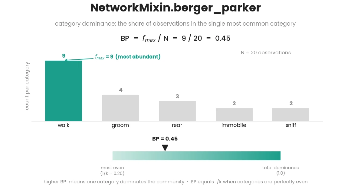
Berger-Parker index for the given one-dimensional array. The Berger-Parker index is a measure of category dominance, calculated as the ratio of the frequency of the most abundant category to the total number of observations. Answer how dominated a cluster or community is by categorical variable.

The Berger-Parker index (BP) is calculated using the formula:

\[BP = \frac{f_{\max}}{N}\]

where: - \(f_{\max}\) is the frequency of the most abundant category, - \(N\) is the total number of observations.

Parameters

x (np.ndarray) – One-dimensional numpy array containing the values for which the Berger-Parker index is calculated.

Return float

Berger-Parker index value for the input array x

Example

>>> x = np.random.randint(0, 25, (100,)).astype(np.float32)
>>> z = NetworkMixin.berger_parker(x=x)

static brillouins_index(x)

Calculate Brillouin’s Diversity Index for a given array of values.

Brillouin’s Diversity Index is a measure of cluster/community diversity that accounts for both richness and evenness of distribution.

Brillouin’s Diversity Index (H) is calculated using the formula:

\[H = \frac{1}{\log(S)} \sum_{i=1}^{S} \frac{N_i(N_i - 1)}{n(n-1)}\]

where: - \(H\) is Brillouin’s Diversity Index, - \(S\) is the total number of unique species, - \(N_i\) is the count of individuals in the i-th species, - \(n\) is the total number of individuals.

Parameters

x (np.array) – One-dimensional numpy array containing the values for which Brillouin’s Index is calculated.

Return float

Brillouin’s Diversity Index value for the input array x

Example

>>> x = np.random.randint(0, 10, (100,))
>>> NetworkMixin.brillouins_index(x)

static create_graph(data)

Create a single undirected graph with single edges from on dictionary.

Parameters

data (Dict[Tuple[str, str], float]) – A dictionary where keys are tuples representing node pairs and values are the corresponding edge weights.

Return nx.Graph

A networkx graph with nodes and edges defined by the input data.

Example

>>> data = {('Animal_1', 'Animal_2'): 1.0, ('Animal_1', 'Animal_3'): 0.2, ('Animal_2', 'Animal_3'): 0.5}
>>> graph = NetworkMixin.create_graph(data=data)

static create_multigraph(data)

Create a multi-graph from a dictionary of node pairs and associated edge weights.

For example, creates a multi-graph where node edges represent animal relationship weights at different timepoints.

Parameters

data (Dict[Tuple[str, str], List[float]]) – A dictionary where keys are tuples representing node pairs, and values are lists of edge weights associated with each pair.

Return nx.MultiGraph

A NetworkX multigraph with nodes and edges specified by the input data. Each edge is labeled and weighted based on the provided information.

Example

>>> data = {('Animal_1', 'Animal_2'): [0, 0, 0, 6], ('Animal_1', 'Animal_3'): [0, 0, 0, 0], ('Animal_1', 'Animal_4'): [0, 0, 0, 0], ('Animal_1', 'Animal_5'): [0, 0, 0, 0], ('Animal_2', 'Animal_3'): [0, 0, 0, 0], ('Animal_2', 'Animal_4'): [5, 0, 0, 2], ('Animal_2', 'Animal_5'): [0, 0, 0, 0], ('Animal_3', 'Animal_4'): [0, 0, 0, 0], ('Animal_3', 'Animal_5'): [0, 2, 22, 0], ('Animal_4', 'Animal_5'): [0, 0, 0, 0]}
>>> NetworkMixin().create_multigraph(data=data)

static girvan_newman(graph, levels=1, most_valuable_edge=None)

Example

>>> graph = NetworkMixin.create_graph({ ('Animal_1', 'Animal_2'): 0.0, ('Animal_1', 'Animal_3'): 0.0, ('Animal_1', 'Animal_4'): 0.0, ('Animal_1', 'Animal_5'): 0.0, ('Animal_2', 'Animal_3'): 1.0, ('Animal_2', 'Animal_4'): 1.0, ('Animal_2', 'Animal_5'): 1.0, ('Animal_3', 'Animal_4'): 1.0, ('Animal_3', 'Animal_5'): 1.0, ('Animal_4', 'Animal_5'): 1.0})
>>> NetworkMixin().girvan_newman(graph=graph, levels = 1)
>>> [({'Animal_1'}, {'Animal_2', 'Animal_3', 'Animal_4', 'Animal_5'})]

static graph_current_flow_closeness_centrality(graph, weights='weight')

Example

>>> graph = NetworkMixin.create_graph(data={('Animal_1', 'Animal_2'): 1.0, ('Animal_1', 'Animal_3'): 0.2, ('Animal_2', 'Animal_3'): 0.5})
>>> NetworkMixin().graph_current_flow_closeness_centrality(graph=graph)

static graph_katz_centrality(graph, weights='weight', alpha=0.85)

Katz centrality is an algorithm in NetworkX that measures the relative influence of a node in a network.

See networkx documentation

Example

>>> graph = NetworkMixin.create_graph(data={('Animal_1', 'Animal_2'): 1.0, ('Animal_1', 'Animal_3'): 0.2, ('Animal_2', 'Animal_3'): 0.5})
>>> NetworkMixin().graph_katz_centrality(graph=graph)

static graph_page_rank(graph, weights='weight', alpha=0.85, max_iter=100)

Calculate the PageRank of nodes in a graph.

Example

>>> graph = NetworkMixin.create_graph(data={('Animal_1', 'Animal_2'): 1.0, ('Animal_1', 'Animal_3'): 0.2, ('Animal_2', 'Animal_3'): 0.5})
>>> NetworkMixin().graph_page_rank(graph=graph)

static margalef_diversification_index(x)

Calculate the Margalef Diversification Index for a given array of values.

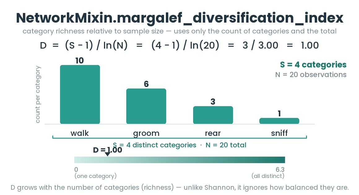
The Margalef Diversification Index is a measure of category diversity. It quantifies the richness of a community/cluster relative to the number of individuals. A high Margalef Diversification Index indicates a high diversity of categories relative to the number of observations. A low Margalef Diversification Index suggests a lower diversity of categories relative to the number of observations.

The Margalef Diversification Index (D) is calculated using the formula:

\[D = \frac{(S - 1)}{\log(N)}\]

where: - \(S\) is the number of unique categories, - \(N\) is the total number of individuals.

Parameters

x (np.array) – One-dimensional numpy array containing nominal values for which the Margalef Diversification Index is calculated.

Return float

Margalef Diversification Index value for the input array x

Example

>>> x = np.random.randint(0, 100, (100,))
>>> NetworkMixin.margalef_diversification_index(x=x)

static menhinicks_index(x)

Calculate the Menhinick’s Index for a given array of values.

Menhinick’s Index is a measure of category richness. It quantifies the number of categories relative to the square root of the total number of observations. A high Menhinick’s Index suggests a high diversity of categories relative to the number of observations. A low Menhinick’s Index indicates a lower diversity of categories relative to the number of observations.

Menhinick’s Index (D) is calculated using the formula:

\[D = \frac{S}{\sqrt{N}}\]

where: - \(S\) is the number of unique categories, - \(N\) is the total number of observations.

param np.array x

One-dimensional numpy array containing the integer values representing nominal values for which Menhinick’s Index is calculated.

return float

Menhinick’s Index value for the input array x

Example

>>> x = np.random.randint(0, 5, (1000,))
>>> NetworkMixin.menhinicks_index(x=x)

static multigraph_page_rank(graph, weights='weight', alpha=0.85, max_iter=100)

Calculate multi-graph PageRank scores for each node in a MultiGraph.

For example, each node-pair in a graph has N undirected edges representing the weighted relationship between the two nodes atobserved point in time. Calculates the page rank of each node at each observed time point.

Parameters

graph (nx.MultiGraph) – The input MultiGraph, created by NetworkMixin.create_multigraph().

Example

>>> multigraph = NetworkMixin().create_multigraph(data={('Animal_1', 'Animal_2'): [0, 0, 0, 6], ('Animal_1', 'Animal_3'): [0, 0, 0, 0], ('Animal_1', 'Animal_4'): [0, 0, 0, 0], ('Animal_1', 'Animal_5'): [0, 0, 0, 0], ('Animal_2', 'Animal_3'): [0, 0, 0, 0], ('Animal_2', 'Animal_4'): [5, 0, 0, 2], ('Animal_2', 'Animal_5'): [0, 0, 0, 0], ('Animal_3', 'Animal_4'): [0, 0, 0, 0], ('Animal_3', 'Animal_5'): [0, 2, 22, 0], ('Animal_4', 'Animal_5'): [0, 0, 0, 0]})
>>> NetworkMixin().multigraph_page_rank(graph=multigraph)
>>> {'Animal_1': [0.06122524589028524, 0.06122524589028524, 0.06122524589028524, 0.32739635847890775], 'Animal_2': [0.06122524589028524, 0.40816213116457223, 0.06122524589028524, 0.442259400816002], 'Animal_3': [0.40816213116457223, 0.06122524589028524, 0.40816213116457223, 0.04545454545454547], 'Animal_4': [0.06122524589028524, 0.40816213116457223, 0.06122524589028524, 0.13943514979599955], 'Animal_5': [0.40816213116457223, 0.06122524589028524, 0.40816213116457223, 0.04545454545454547]}

static shannon_diversity_index(x)

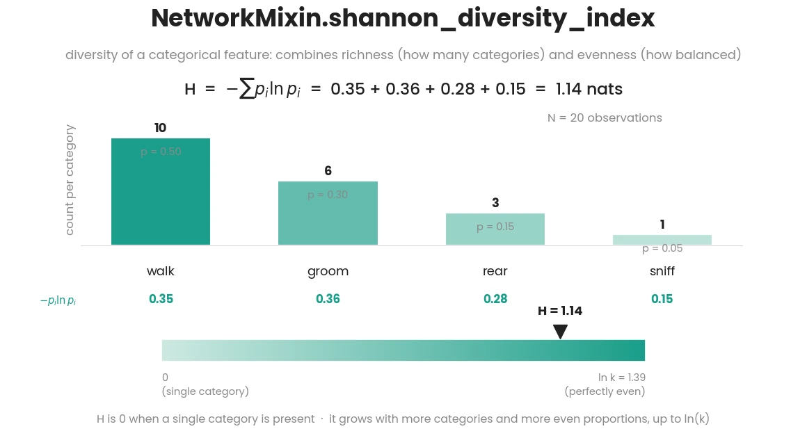
Calculate the Shannon Diversity Index for a given array of categories. The Shannon Diversity Index is a measure of diversity in a categorical feature, taking into account both the number of different categories (richness) and their relative abundances (evenness). Answer how homogenous a cluster or community is for categorical variable. A low value indicates that one or a few categories dominate.

\[H = -\sum_{i=1}^{n} (p_i \cdot \log(p_i))\]

where: - \(p_i\) is the proportion of individuals belonging to the i-th category, - \(n\) is the total number of categories.

Parameters

x (np.ndarray) – One-dimensional numpy array containing the categories for which the Shannon Diversity Index is calculated.

Return float

Shannon Diversity Index value for the input array x

Example

>>> x = np.random.randint(0, 100, (100, ))
>>> NetworkMixin.shannon_diversity_index(x=x)

static simpson_index(x)

Calculate Simpson’s diversity index for a given array of values.

Simpson’s diversity index is a measure of diversity that takes into account the number of different categories present in the input data as well as the relative abundance of each category. Answer how homogenous a cluster or community is for categorical input variable.

\[D = \frac{\sum(n(n-1))}{N(N-1)}\]

where: - \(n\) is the number of individuals of a particular category, - \(N\) is the total number of individuals, - \(\sum\) represents the sum over all categories.

Parameters

x (np.ndarray) – 1-dimensional numpy array containing the values representing categories for which Simpson’s index is calculated.

Return float

Simpson’s diversity index value for the input array x

static sorensen_dice_coefficient(x, y)

Calculate Sørensen’s Similarity Index between two communities/clusters.

The Sørensen similarity index, also known as the overlap index, quantifies the overlap between two populations by comparing the number of shared categories to the total number of categories in both populations. It ranges from zero, indicating no overlap, to one, representing perfect overlap

Sørensen’s Similarity Index (S) is calculated using the formula:

\[S = \frac{2 \times |X \cap Y|}{|X| + |Y|}\]

where: - \(S\) is Sørensen’s Similarity Index, - \(X\) and \(Y\) are the sets representing the categories in the first and second communities, respectively, - \(|X \cap Y|\) is the number of shared categories between the two communities, - \(|X|\) and \(|Y|\) are the total number of categories in the first and second communities, respectively.

Parameters

• x – 1D numpy array with nominal values for the first cluster/community.

• y – 1D numpy array with nominal values for the second cluster/community.

Returns

Sørensen’s Similarity Index between x and y.

Example

>>> x = np.random.randint(0, 10, (100,))
>>> y = np.random.randint(0, 10, (100,))
>>> NetworkMixin.sorensen_dice_coefficient(x=x, y=y)

static visualize(graph, save_path=None, node_size=25.0, palette='magma', node_shape='dot', smooth_type='dynamic', img_size=(500, 500), seed=None)

Visualizes a network graph using the vis.js library and saves the result as an HTML file.

Note

Multi-networks created by simba.mixins.network_mixin.create_multigraph can be a little messy to look at. Instead, creates separate objects and files with single edges from each time-point.

Parameters

• graph (Union[nx.Graph, nx.MultiGraph]) – The input graph to be visualized.

• save_path (Optional[Union[str, os.PathLike]]) – The path to save the HTML file. If multi-graph, pass a directory path. If None, the graph(s) are returned but not saved.

• node_size (Optional[Union[float, Dict[str, float]]]) – The size of nodes. Can be a single float or a dictionary mapping node names to their respective sizes. Default: 25.0.

• palette (Optional[Union[str, Dict[str, str]]]) – The color palette for nodes. Can be a single string representing a palette name or a dictionary mapping node names to their respective colors. Default; magma.

• img_size (Optional[Tuple[int, int]]) – The size of the resulting image in pixels, represented as (width, height). Default: 500x500.

• node_shape (Optional[Literal['dot', 'ellipse', 'circle']]) – The shape of the nodes. Default: dot.

• smooth_type (Optional[Literal]) – The dynamics of the interactive graph.

Example

>>> graph = NetworkMixin.create_graph(data={('Animal_1', 'Animal_2'): 1.0, ('Animal_1', 'Animal_3'): 0.2, ('Animal_2', 'Animal_3'): 0.5})
>>> graph_pg = NetworkMixin.visualize(graph=graph, node_size={'Animal_1': 10, 'Animal_2': 26, 'Animal_3': 50}, save_path='/Users/simon/Downloads/graph.html', node_shape='box', palette='spring')
>>> multigraph = NetworkMixin().create_multigraph(data={('Animal_1', 'Animal_2'): [0, 0, 0, 6], ('Animal_1', 'Animal_3'): [0, 0, 0, 0], ('Animal_1', 'Animal_4'): [0, 0, 0, 0], ('Animal_1', 'Animal_5'): [0, 0, 0, 0], ('Animal_2', 'Animal_3'): [0, 0, 0, 0], ('Animal_2', 'Animal_4'): [5, 0, 0, 2], ('Animal_2', 'Animal_5'): [0, 0, 0, 0], ('Animal_3', 'Animal_4'): [0, 0, 0, 0], ('Animal_3', 'Animal_5'): [0, 2, 22, 0], ('Animal_4', 'Animal_5'): [0, 0, 0, 0]})
>>> graph_pg = NetworkMixin.visualize(graph=multigraph, node_size={'Animal_1': 10, 'Animal_2': 26, 'Animal_3': 50, 'Animal_4': 50, 'Animal_5': 50}, save_path='/Users/simon/Downloads/graphs', node_shape='box', palette='spring', smooth_type='diagonalCross')