Time-series transformations

Time-series statistics mixin

class simba.mixins.timeseries_features_mixin.TimeseriesFeatureMixin[source]

Time-series methods focused on signal complexity in sliding windows. Mainly in time-domain - fft methods (through e.g. scipy) I’ve found so far has not been fast enough for rolling windows in large datasets.

Note

Many method has numba typed signatures to decrease compilation time through reduced type inference. Make sure to pass the correct dtypes as indicated by signature decorators.

Important

See references for mature packages computing more extensive timeseries measurements

1: cesium.
2: eeglib.
3: antropy.
4: tsfresh.
5: pycaret.
6: stumpy.

static acceleration(data, pixels_per_mm, fps, time_window=1, unit='mm')[source]

Compute framewise acceleration from a movement (framewise-distance) signal.

Given a 1D array of framewise euclidean distances - the per-frame movement of a body-part, in pixels - this first converts movement to speed in the requested unit per second, then returns the rate of change of that speed over a rolling time_window: the acceleration. Positive values mean the body-part is speeding up, negative values mean it is slowing down.

The computation is:

\[v(t) = \frac{\text{data}(t)\, \cdot\, \text{fps}}{\text{pixels\_per\_mm}\, \cdot\, c_{\text{unit}}}, \qquad a(t) = \frac{v(t) - v(t - w)}{\text{time\_window}}\]

where \(v(t)\) is speed at frame \(t\) (unit/s), \(w = \mathrm{round}(\text{time\_window} \cdot \text{fps})\) is the window length in frames, and \(c_{\text{unit}}\) converts millimeters to the chosen unit (mm = 1, cm = 10, dm = 100, m = 1000). The first \(w\) frames have no earlier reference and are returned as 0.

Note

time_window sets both the interval over which the velocity change is measured and the value the change is divided by, so the result is a true per-second rate (unit/s²) regardless of the window length. Use unit to change the length unit (mm, cm, dm, m).

Parameters

data (np.ndarray) – 1D array of framewise euclidean distances (per-frame body-part movement, in pixels).
pixels_per_mm (float) – Pixels per millimeter of the recorded video.
fps (int) – Frames per second (FPS) of the recorded video.
time_window (float) – Rolling time window in seconds over which the velocity change is measured. Default is 1.0.
unit (Literal['mm', 'cm', 'dm', 'm']) – Length unit of the result (millimeter, centimeter, decimeter, or meter). Default millimeters.

Returns

Array of accelerations (unit/s²), one per frame; the first round(time_window * fps) entries are 0.

Return type

np.ndarray

Example

>>> data = np.array([0, 1, 1, 1, 2, 2, 2, 1, 1, 0]).astype(np.float32)
>>> TimeseriesFeatureMixin.acceleration(data=data, pixels_per_mm=1.0, fps=2, time_window=1.0)
>>> [ 0.,  0.,  2.,  0.,  2.,  2.,  0., -2., -2., -2.]

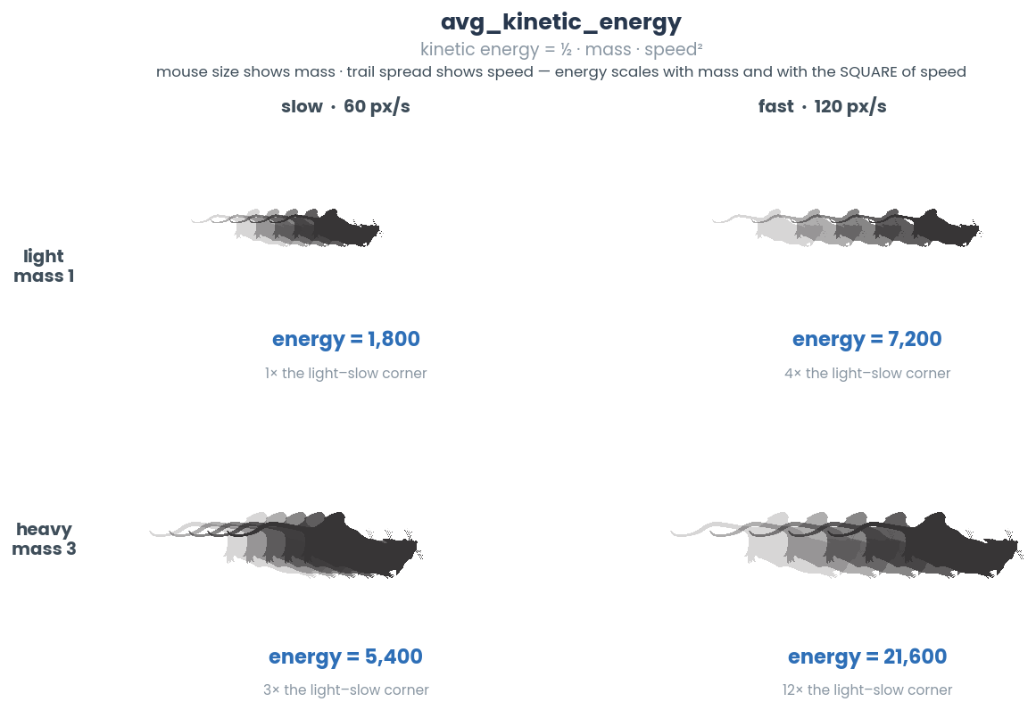
static avg_kinetic_energy(x, mass, sample_rate)[source]

Calculate the average kinetic energy of an object based on its velocity.

Parameters

x (np.ndarray) – A 2D NumPy array of shape (n, 2), where each row contains the x and y position coordinates of the object at each time step.
mass (float) – The mass of the object.
sample_rate (float) – The sampling rate (Hz), i.e., the number of data points per second.

Returns

The average kinetic energy of the animal.

Return type

float

Example

>>> x = np.random.randint(0, 500, (200, 2))
>>> TimeseriesFeatureMixin.avg_kinetic_energy(x=x, mass=35, sample_rate=30)

static benford_correlation(data)[source]

Jitted compute of the correlation between the Benford’s Law distribution and the first-digit distribution of given data.

Benford’s Law describes the expected distribution of leading (first) digits in many real-life datasets. This function calculates the correlation between the expected Benford’s Law distribution and the actual distribution of the first digits in the provided data.

Note

Adapted from tsfresh.

The returned correlation values are calculated using Pearson’s correlation coefficient.

Parameters: data (np.ndarray) – The input 1D array containing the time series data.
Returns: The correlation coefficient between the Benford’s Law distribution and the first-digit distribution in the input data. A higher correlation value suggests that the data follows the expected distribution more closely.
Return type: float
Examples

>>> data = np.array([1, 8, 2, 10, 8, 6, 8, 1, 1, 1]).astype(np.float32)
>>> TimeseriesFeatureMixin().benford_correlation(data=data)
>>> 0.6797500374831786

static crossings(data, val)[source]

Jitted compute of the count in time-series where sequential values crosses a defined value.

Parameters

data (np.ndarray) – Time-series data.
val (float) – Cross value. E.g., to count the number of zero-crossings, pass 0.

Return int

Count of events where sequential values crosses val.

Example

>>> data = np.array([3.9, 7.5,  4.2, 6.2, 7.5, 3.9, 6.2, 6.5, 7.2, 9.5]).astype(np.float32)
>>> TimeseriesFeatureMixin().crossings(data=data, val=7)
>>> 5

static dominant_frequencies(data, fps, k, window_function=None)[source]: Find the K dominant frequencies within a feature vector

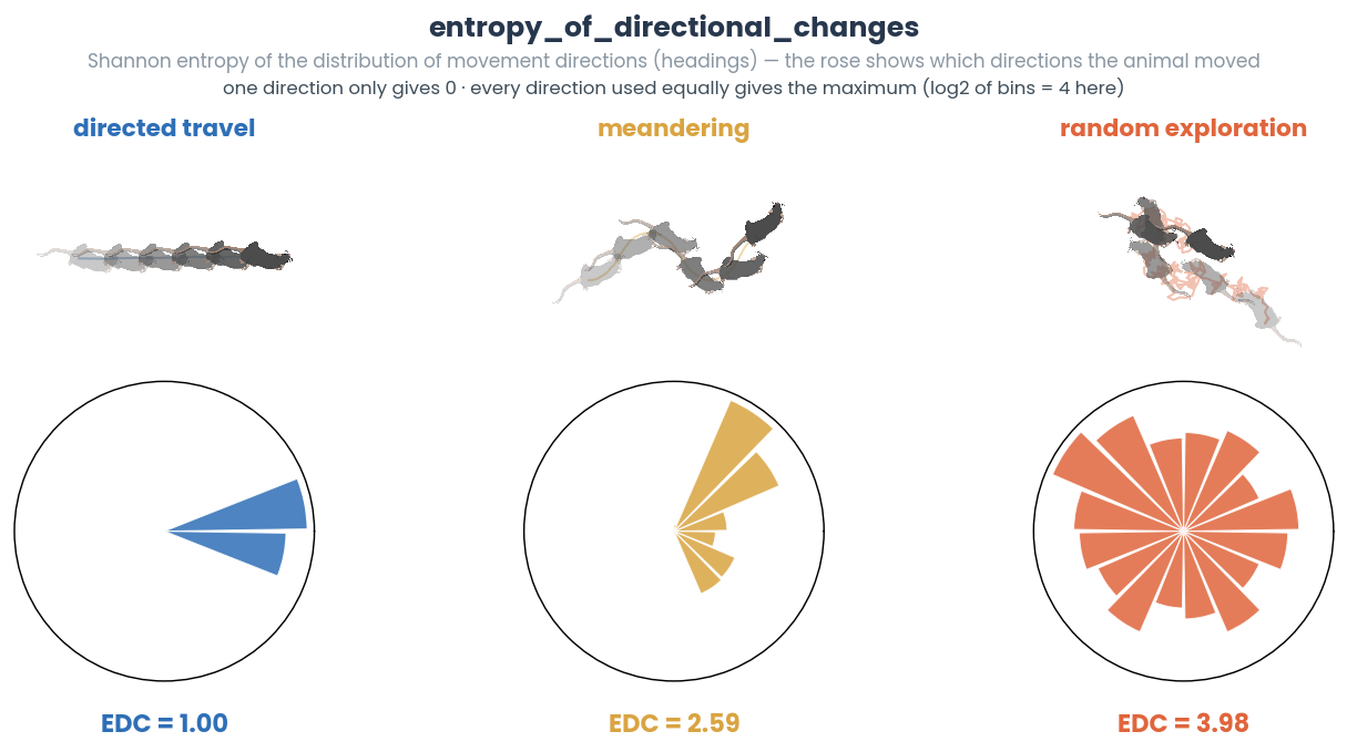
static entropy_of_directional_changes(x, bins=16)[source]

Computes the Entropy of Directional Changes (EDC) of a path represented by an array of points.

The output value ranges from 0 to log2(bins).

The Entropy of Directional Changes quantifies the unpredictability or randomness of the directional changes in a given path. Higher entropy indicates more variation in the directions of the movement, while lower entropy suggests more linear or predictable movement.

The function works by calculating the change in direction between consecutive points, discretizing those changes into bins, and then computing the Shannon entropy based on the probability distribution of the directional changes.

\[H = -\sum_{i=1}^{\text{bins}} p_i \log_2(p_i)\]

Where:

\(p_i\) is the probability of the direction falling into the \(i\)-th bin.
\(\text{bins}\) represents the total number of bins for discretizing the directional changes.

Parameters

x (np.ndarray) – A 2D array of shape (N, 2) representing the path, where N is the number of points and each point has two spatial coordinates (e.g., x and y for 2D space). The path should be in the form of an array of consecutive (x, y) points.
bins (int) – The number of bins to discretize the directional changes. Default is 16 bins for angles between 0 and 360 degrees. A larger number of bins will increase the precision of direction change measurement.

Returns

The entropy of the directional changes in the path. A higher value indicates more unpredictable or random direction changes, while a lower value indicates more predictable or linear movement.

Return type

float

Example

>>> x = np.random.randint(0, 500, (100, 2))
>>> TimeseriesFeatureMixin.entropy_of_directional_changes(x, 3)

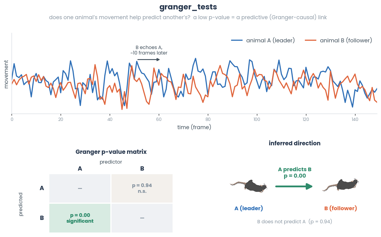
static granger_tests(data, variables, lag, test='ssr_chi2test')[source]

Perform Granger causality tests between pairs of variables in a DataFrame.

This function computes Granger causality tests between pairs of variables in a DataFrame using the statsmodels library. The Granger causality test assesses whether one time series variable (predictor) can predict another time series variable (outcome). This test can help determine the presence of causal relationships between variables.

Note

Modified from Selva Prabhakaran.

Example

>>> x = np.random.randint(0, 50, (100, 2))
>>> data = pd.DataFrame(x, columns=['r', 'k'])
>>> TimeseriesFeatureMixin.granger_tests(data=data, variables=['r', 'k'], lag=4, test='ssr_chi2test')
>>>     r           k
>>>     r  1.0000  0.4312
>>>     k  0.3102  1.0000

static higuchi_fractal_dimension(data, kmax=10)[source]

Jitted compute of the Higuchi Fractal Dimension of a given time series data. The Higuchi Fractal Dimension provides a measure of the fractal complexity of a time series.

The maximum value of k used in the calculation. Increasing kmax considers longer sequences of data, providing a more detailed analysis of fractal complexity. Default is 10.

Parameters

data (np.ndarray) – A 1-dimensional numpy array containing the time series data.
kmax (int) – The maximum value of k used in the calculation. Increasing kmax considers longer sequences of data, providing a more detailed analysis of fractal complexity. Default is 10.

Returns

The Higuchi Fractal Dimension of the input time series.

Return type

float

Note

Adapted from eeglib.

\[HFD = \frac{\log(N)}{\log(N) + \log\left(\frac{N}{N + 0.4 \cdot zC}\right)}\]

Example

>>> t = np.linspace(0, 50, int(44100 * 2.0), endpoint=False)
>>> sine_wave = 1.0 * np.sin(2 * np.pi * 1.0 * t).astype(np.float32)
>>> sine_wave = (sine_wave - np.min(sine_wave)) / (np.max(sine_wave) - np.min(sine_wave))
>>> TimeseriesFeatureMixin().higuchi_fractal_dimension(data=data, kmax=10)
>>> 1.0001506805419922
>>> np.random.shuffle(sine_wave)
>>> TimeseriesFeatureMixin().higuchi_fractal_dimension(data=data, kmax=10)
>>> 1.9996402263641357

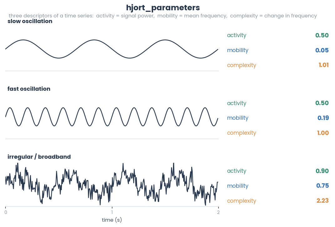
static hjort_parameters(data)[source]

Jitted compute of Hjorth parameters for a given time series data. Hjorth parameters describe mobility, complexity, and activity of a time series.

Parameters: data (numpy.ndarray) – A 1-dimensional numpy array containing the time series data.
Returns: A tuple containing the following Hjorth parameters: - activity (float): The activity of the time series, which is the variance of the input data. - mobility (float): The mobility of the time series, calculated as the square root of the variance of the first derivative of the input data divided by the variance of the input data. - complexity (float): The complexity of the time series, calculated as the square root of the variance of the second derivative of the input data divided by the variance of the first derivative, and then divided by the mobility.
Return type

Note

A constant first derivative (e.g. a perfectly linear ramp) yields var(dx) == 0; in that degenerate case the function returns (0, 0, 0) to avoid division by zero.

Example

>>> data = np.array([1.0, 3.0, 2.0, 6.0, 4.0, 5.0], dtype=np.float32)
>>> TimeseriesFeatureMixin().hjort_parameters(data)
>>> (2.9166667, 1.2503713, 1.6617813)  # (activity, mobility, complexity)

\(mobility = \sqrt{\frac{dx_{var}}{x_{var}}}\)

\(complexity = \sqrt{\frac{ddx_{var}}{dx_{var}} / mobility}\)

static line_length(data)[source]

Calculate the line length of a 1D array.

Line length is a measure of signal complexity and is computed by summing the absolute differences between consecutive elements of the input array. Used in EEG analysis and other signal processing applications to quantify variations in the signal.

\[LL = \sum_{i=1}^{N-1} |x[i] - x[i-1]|\]

where: \(LL\) is the line length. \(N\) is the number of elements in the input data array. \(x[i]\) represents the value of the data at index i.

Parameters: data (numpy.ndarray) – The 1D array for which the line length is to be calculated.
Returns: The line length of the input array, indicating its complexity.
Return type: float
Example

>>> data = np.array([1, 4, 2, 3, 5, 6, 8, 7, 9, 10]).astype(np.float32)
>>> TimeseriesFeatureMixin().line_length(data=data)
>>> 12.0

static linearity_index(x)[source]

Calculates the straightness (linearity) index of a path.

\[\text{linearity\_index} = \frac{\text{straight\_line\_distance}}{\text{path\_length}}\]

Where:

\(\text{straight\_line\_distance}\) is the Euclidean distance between the starting and ending points of the path.
\(\text{path\_length}\) is the sum of Euclidean distances between consecutive points along the path.

Parameters: x (np.ndarray) – An (N, M) array representing the path, where N is the number of points and M is the number of spatial dimensions (e.g., 2 for 2D or 3 for 3D). Each row represents the coordinates of a point along the path.
Returns: The straightness index of the path, a value between 0 and 1, where 1 indicates a perfectly straight path.
Return type: float
Example

>>> x = np.array([[0, 0], [1, 1], [2, 2], [3, 3], [4, 4], [5, 5]])
>>> TimeseriesFeatureMixin.linearity_index(x=x)
>>> x = np.random.randint(0, 100, (100, 2))
>>> TimeseriesFeatureMixin.linearity_index(x=x)

static local_maxima_minima(data, maxima=True)[source]

Jitted compute of the local maxima or minima defined as values which are higher or lower than immediately preceding and proceeding time-series neighbors, repectively. Returns 2D np.ndarray with columns representing idx and values of local maxima.

Parameters

data (np.ndarray) – Time-series data.
maxima (bool) – If True, returns maxima. Else, minima.

Return np.ndarray

2D np.ndarray with columns representing idx in input data in first column and values of local maxima in second column

Example

>>> data = np.array([3.9, 7.5,  4.2, 6.2, 7.5, 3.9, 6.2, 6.5, 7.2, 9.5]).astype(np.float32)
>>> TimeseriesFeatureMixin().local_maxima_minima(data=data, maxima=True)
>>> [[1, 7.5], [4, 7.5], [9, 9.5]]
>>> TimeseriesFeatureMixin().local_maxima_minima(data=data, maxima=False)
>>> [[0, 3.9], [2, 4.2], [5, 3.9]]

static longest_strike(data, threshold, above=True)[source]

Jitted compute of the length of the longest consecutive sequence of values in the input data that either exceed or fall below a specified threshold.

Parameters

data (np.ndarray) – The input 1D NumPy array containing the values to be analyzed.
threshold (float) – The threshold value used for the comparison.
above (bool) – If True, the function looks for strikes where values are above or equal to the threshold. If False, it looks for strikes where values are below or equal to the threshold.

Returns

The length of the longest strike that satisfies the condition.

Return type

int

Example

>>> data = np.array([1, 8, 2, 10, 8, 6, 8, 1, 1, 1]).astype(np.float32)
>>> TimeseriesFeatureMixin().longest_strike(data=data, threshold=7, above=True)
>>> 2
>>> TimeseriesFeatureMixin().longest_strike(data=data, threshold=7, above=False)
>>> 3

static mean_squared_jerk(x, time_step, sample_rate)[source]

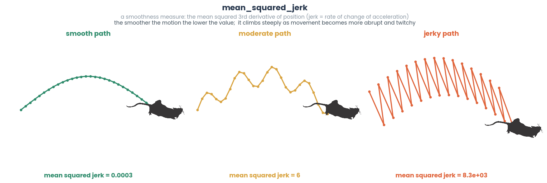
Calculate the Mean Squared Jerk (MSJ) for a given set of 2D positions over time.

The Mean Squared Jerk is a measure of the smoothness of movement, calculated as the mean of squared third derivatives of the position with respect to time. It provides an indication of how abrupt or smooth a trajectory is, with higher values indicating more erratic movements.

The formula for Mean Squared Jerk is:

\[\text{MSJ} = \frac{1}{N - 3} \sum_{i=1}^{N-3} \| \frac{d^3 x_i}{dt^3} \|^2\]

where \(N\) is the number of points, \(x_i\) represents the position at each point, and \(\frac{d^3 x_i}{dt^3}\) is the third derivative of the position with respect to time.

Parameters

x (np.ndarray) – A 2D array where each row represents the [x, y] position at a time step.
time_step (float) – The time difference between successive positions in seconds.
sample_rate (float) – The rate at which the positions are sampled (samples per second).

Returns

The computed Mean Squared Jerk for the input trajectory data.

Return type

float

Example I

>>> x = np.random.randint(0, 500, (100, 2))
>>> TimeseriesFeatureMixin.mean_squared_jerk(x=x, time_step=1.0, sample_rate=30)

static momentum_magnitude(x, mass, sample_rate)[source]

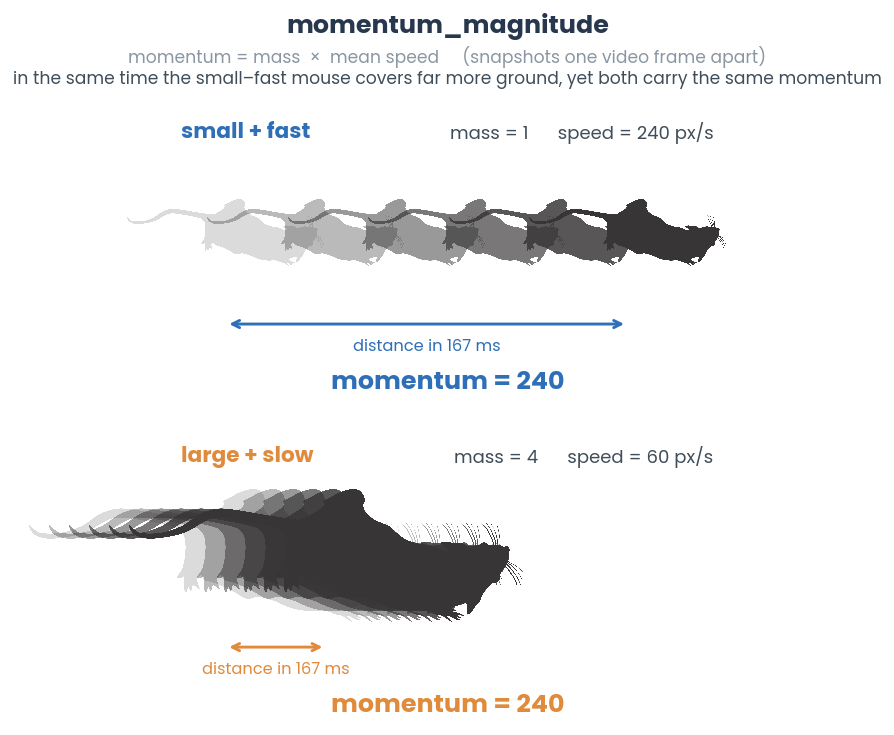
Compute the magnitude of momentum given 2D positional data and mass.

Parameters

x (np.ndarray) – 2D array of shape (n_samples, 2) representing positions.
mass (float) – Mass of the object.
sample_rate (float) – Sampling rate in FPS.

Returns

Magnitude of the momentum.

Return type

float

static path_aspect_ratio(x, px_per_mm)[source]

Calculates the aspect ratio of the bounding box that encloses a given path.

Parameters

x (np.ndarray) – A 2D array of shape (N, 2) representing the path, where N is the number of points and each point has two spatial coordinates (e.g., x and y for 2D space). The path should be in the form of an array of consecutive (x, y) points.
px_per_mm (float) – Conversion factor representing the number of pixels per millimeter

Returns

The aspect ratio of the bounding box enclosing the path. If the width or height of the bounding box is zero (e.g., if all points are aligned vertically or horizontally), returns -1.

Return type

float

Example

>>> x = np.random.randint(0, 500, (10, 2))
>>> TimeseriesFeatureMixin.path_aspect_ratio(x=x)

static path_curvature(x, agg_type='mean')[source]

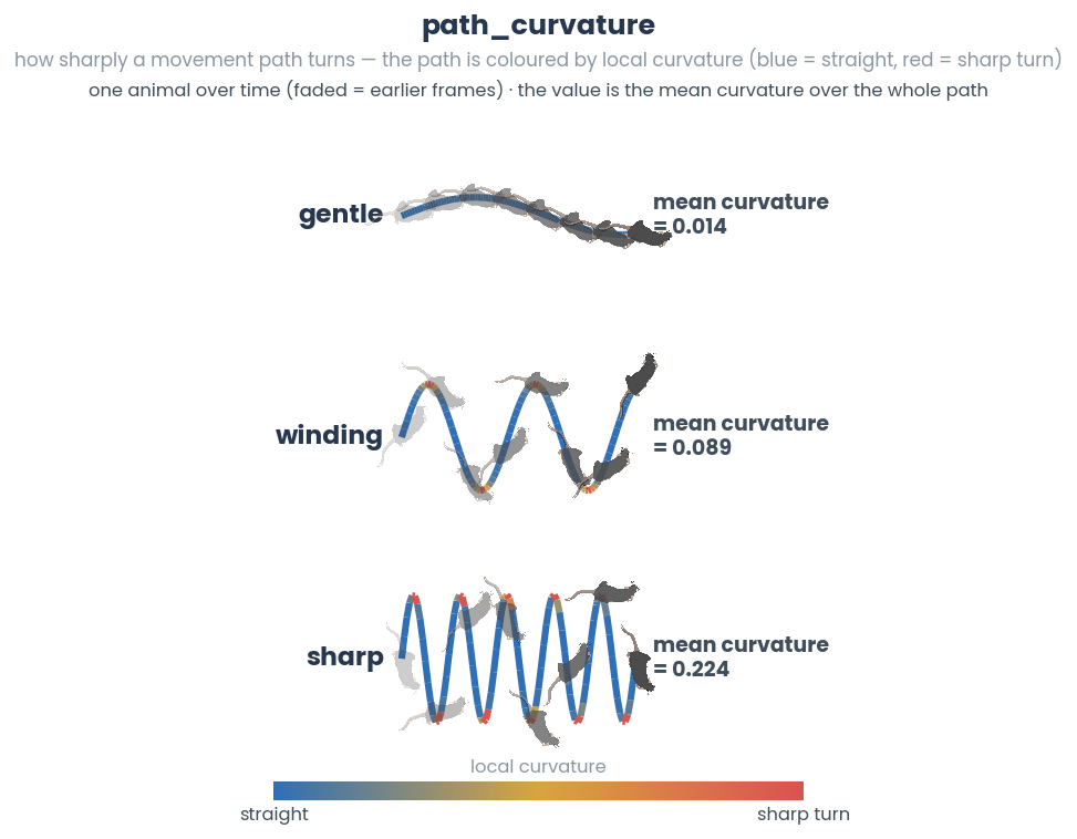
Calculate aggregate curvature of a 2D path given an array of points.

The curvature quantifies the change in direction along the path. Higher curvature values indicate sharper turns, while lower values suggest a straighter path. The function aggregates curvature values across the path using the specified statistic.

\[\kappa = \frac{|x' y'' - y' x''|}{(x'^2 + y'^2)^{3/2}}\]

Where: - \(x'\) and \(y'\) are the first derivatives (differences) of the x and y coordinates, respectively. - \(x''\) and \(y''\) are the second derivatives (differences of differences) of the x and y coordinates.

Parameters

x – A 2D numpy array of shape (N, 2), where N is the number of points and each row is (x, y).
agg_type (Literal['mean', 'median', 'max']) – The type of summary statistic to return. Options are ‘mean’, ‘median’, or ‘max’.

Returns

A single float value representing the path curvature based on the specified summary type.

Return type

float

Example

>>> x = np.array([[0, 0], [1, 0.1], [2, 0.2], [3, 0.3], [4, 0.4]])
>>> low = TimeseriesFeatureMixin.path_curvature(x)
>>> x = np.array([[0, 0], [1, 1], [2, 0], [3, 1], [4, 0]])
>>> high = TimeseriesFeatureMixin.path_curvature(x)

static percent_beyond_n_std(data, n)[source]

Jitted compute of the ratio of values in time-series more than N standard deviations from the mean of the time-series.

Note

Adapted from cesium.

Oddetity: mean calculation is incorrect if passing float32 data but correct if passing float64.

Parameters

data (np.ndarray) – 1D array representing time-series.
n (float) – Standard deviation cut-off.

Returns

Ratio of values in data that fall more than n standard deviations from mean of data.

Return type

float

Examples

>>> data = np.array([3.9, 7.5,  4.2, 6.2, 7.5, 3.9, 6.2, 6.5, 7.2, 9.5]).astype(np.float32)
>>> TimeseriesFeatureMixin().percent_beyond_n_std(data=data, n=1)
>>> 0.1

static percent_in_percentile_window(data, upper_pct, lower_pct)[source]

Jitted compute of the ratio of values in time-series that fall between the upper and lower percentile.

Note

Adapted from cesium.

Parameters

data (np.ndarray) – 1D array of representing time-series.
upper_pct (int) – Upper-boundary percentile.
lower_pct (int) – Lower-boundary percentile.

Returns

Ratio of values in data that fall within upper_pct and lower_pct percentiles.

Return type

float

Example

>>> data = np.array([3.9, 7.5,  4.2, 6.2, 7.5, 3.9, 6.2, 6.5, 7.2, 9.5]).astype(np.float32)
>>> TimeseriesFeatureMixin().percent_in_percentile_window(data, upper_pct=70, lower_pct=30)
>>> 0.4

static percentile_difference(data, upper_pct, lower_pct)[source]

Jitted compute of the difference between the upper and lower percentiles of the data as a percentage of the median value. Helps understand the spread or variability of the data within specified percentiles.

Note

Adapted from cesium.

Parameters

data (np.ndarray) – 1D array of representing time-series.
upper_pct (int) – Upper-boundary percentile.
lower_pct (int) – Lower-boundary percentile.

Returns

The difference between the upper and lower percentiles of the data as a percentage of the median value.

Return type

float

Examples

>>> data = np.array([3.9, 7.5,  4.2, 6.2, 7.5, 3.9, 6.2, 6.5, 7.2, 9.5]).astype(np.float32)
>>> TimeseriesFeatureMixin().percentile_difference(data=data, upper_pct=95, lower_pct=5)
>>> 0.7401574764125177

static permutation_entropy(data, dimension, delay)[source]

Calculate the permutation entropy of a time series.

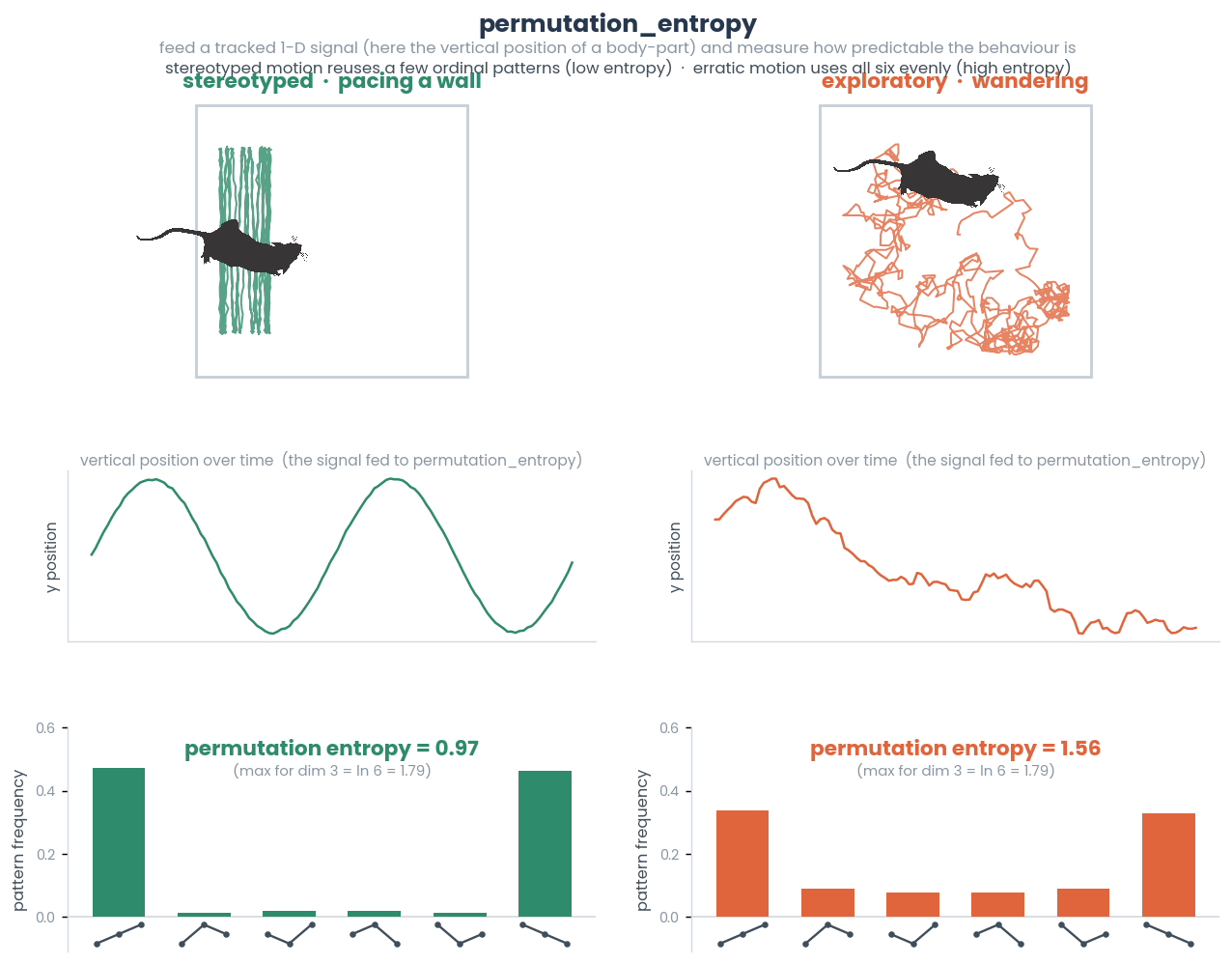
Permutation entropy is a measure of the complexity of a time series data by quantifying the irregularity and unpredictability of its order patterns. It is computed based on the frequency of unique order patterns of a given dimension in the time series data.

The permutation entropy (PE) is calculated using the following formula:

\[PE = - \sum(p_i \log(p_i))\]

where:: \(PE\) is the permutation entropy. \(p_i\) is the probability of each unique order pattern.

Parameters

data (numpy.ndarray) – The time series data for which permutation entropy is calculated.
dimension (int) – It specifies the length of the order patterns to be considered.
delay (int) – Time delay between elements in an order pattern.

Returns

The permutation entropy of the time series, indicating its complexity and predictability. A higher permutation entropy value indicates higher complexity and unpredictability in the time series.

Return type

float

Example

>>> t = np.linspace(0, 50, int(44100 * 2.0), endpoint=False)
>>> sine_wave = 1.0 * np.sin(2 * np.pi * 1.0 * t).astype(np.float32)
>>> TimeseriesFeatureMixin().permutation_entropy(data=sine_wave, dimension=3, delay=1)
>>> 0.701970058666407
>>> np.random.shuffle(sine_wave)
>>> TimeseriesFeatureMixin().permutation_entropy(data=sine_wave, dimension=3, delay=1)
>>> 1.79172449934604

static petrosian_fractal_dimension(data)[source]

Calculate the Petrosian Fractal Dimension (PFD) of a given time series data. The PFD is a measure of the irregularity or self-similarity of a time series. Larger values indicate higher complexity. Lower values indicate lower complexity.

Note

The PFD is computed based on the number of sign changes in the first derivative of the time series. If the input data is empty or no sign changes are found, the PFD is returned as -1.0. Adapted from eeglib. Adapted from eeglib.

\[PFD = \frac{\log_{10}(N)}{\log_{10}(N) + \log_{10}\left(\frac{N}{N + 0.4 \cdot zC}\right)}\]

Parameters: data (np.ndarray) – A 1-dimensional numpy array containing the time series data.
Returns: The Petrosian Fractal Dimension of the input time series.
Return type: float
Examples

>>> t = np.linspace(0, 50, int(44100 * 2.0), endpoint=False)
>>> sine_wave = 1.0 * np.sin(2 * np.pi * 1.0 * t).astype(np.float32)
>>> TimeseriesFeatureMixin().petrosian_fractal_dimension(data=sine_wave)
>>> 1.0000398187022719
>>> np.random.shuffle(sine_wave)
>>> TimeseriesFeatureMixin().petrosian_fractal_dimension(data=sine_wave)
>>> 1.0211625348743218

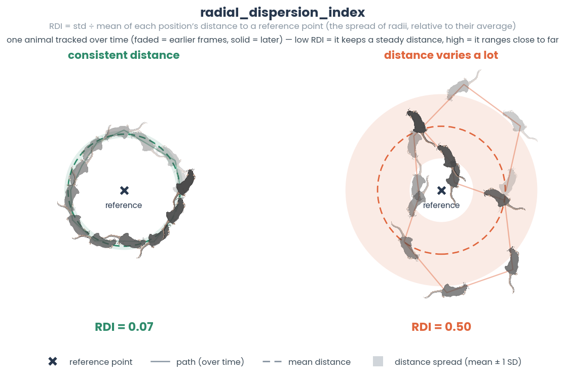
static radial_dispersion_index(x, reference_point)[source]

Compute the Radial Dispersion Index (RDI) for a set of points relative to a reference point.

The RDI quantifies the variability in radial distances of points from the reference point, normalized by the mean radial distance. For example, the radial dispersion from an ROI center.

Parameters

x (np.ndarray) – 2-dimensional numpy array representing the input data with shape (n, m), where n is the number of frames and m is the coordinates.
reference_point (np.ndarray) – A 1D array of shape (n_dimensions,) representing the reference point with respect to which the radial dispertion index is calculated.

Return type

float

Example

>>> points = np.random.randint(0, 1000, (100000, 2))
>>> reference_point = np.mean(points, axis=0)
>>> TimeseriesFeatureMixin.radial_dispersion_index(x=points, reference_point=reference_point)

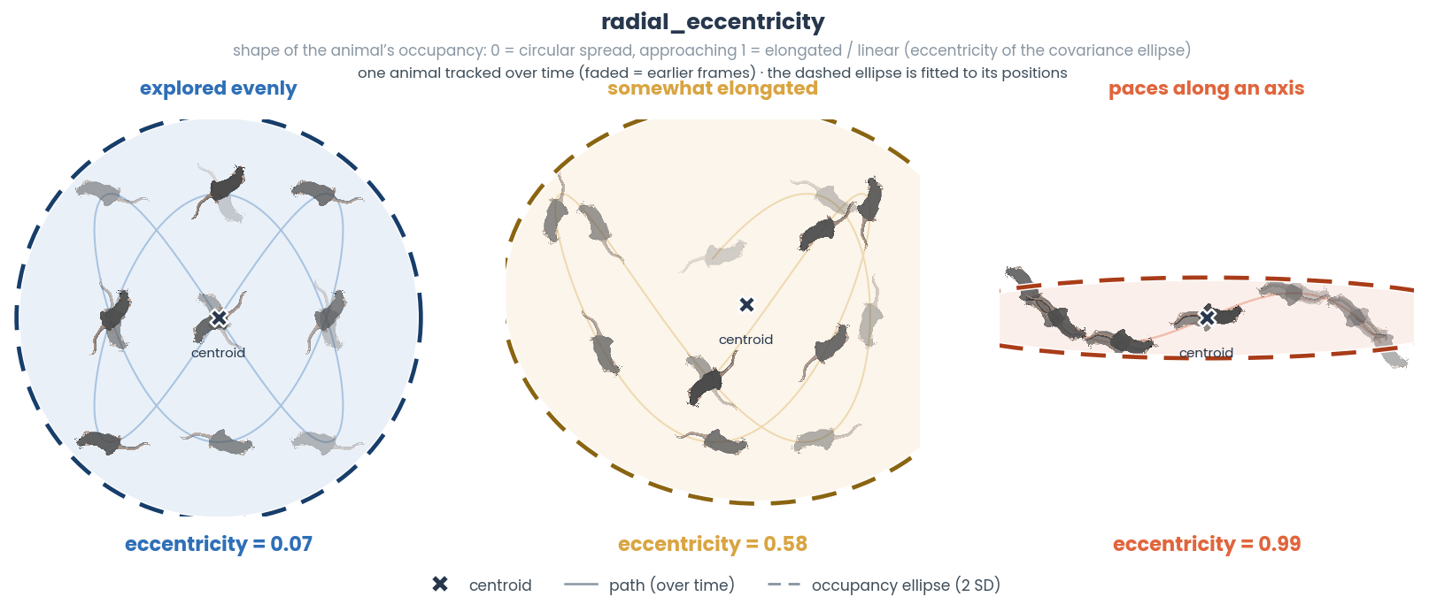
static radial_eccentricity(x, reference_point)[source]

Compute the radial eccentricity of a set of points relative to a reference point.

Radial eccentricity quantifies the degree of elongation in the spatial distribution of points. The value ranges between 0 and 1, where: - 0 indicates a perfectly circular distribution. - Values approaching 1 indicate a highly elongated or linear distribution.

Parameters

x (np.ndarray) – 2-dimensional numpy array representing the input data with shape (n, m), where n is the number of frames and m is the coordinates.
data (np.ndarray) – A 1D array of shape (n_dimensions,) representing the reference point with respect to which the radial eccentricity is calculated.

Example

>>> points = np.random.randint(0, 1000, (100000, 2))
>>> reference_point = np.mean(points, axis=0)
>>> TimeseriesFeatureMixin.radial_eccentricity(x=points, reference_point=reference_point)

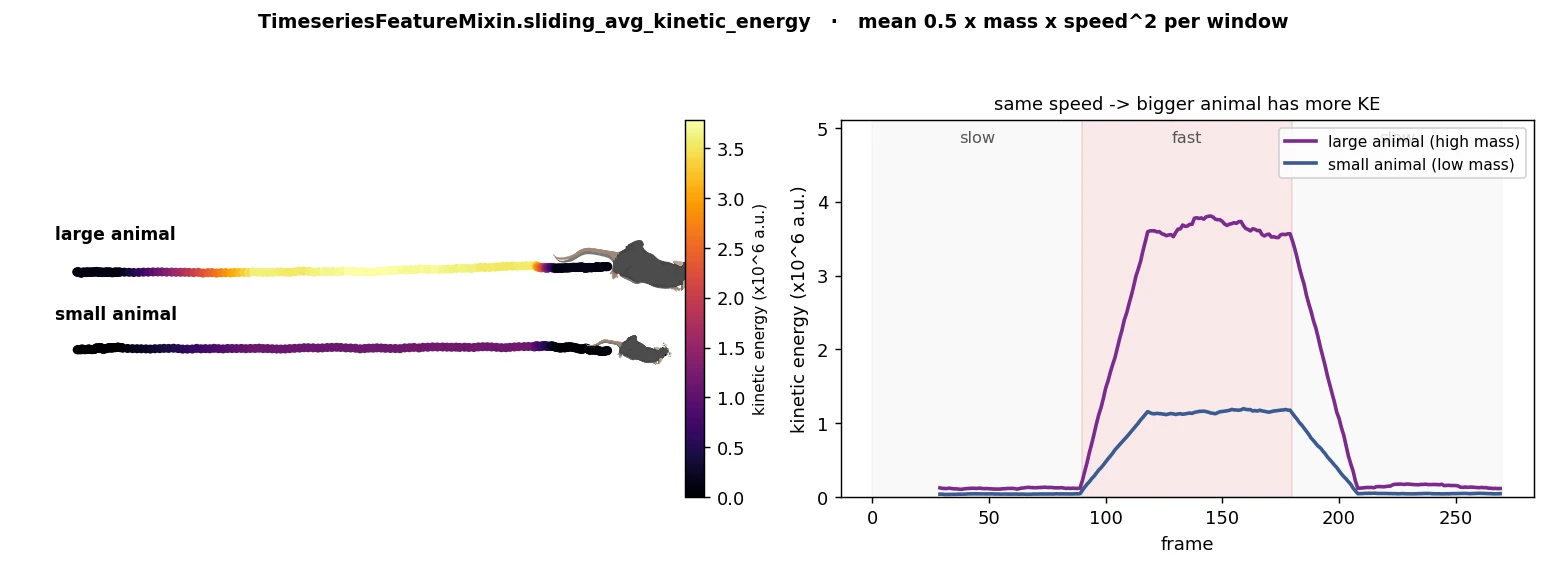
static sliding_avg_kinetic_energy(x, mass, sample_rate, time_window)[source]

Calculate the sliding average kinetic energy of an object over a specified time window.

This function computes the kinetic energy of an object based on its position and mass. The calculation is performed over a sliding time window, returning an array of average kinetic energy values for each valid frame.

Parameters

x (np.ndarray) – A 2D NumPy array of shape (n, 2), where each row contains the x and y position coordinates of the object at each time step.
mass (np.ndarray) – A 1D NumPy array of shape (n,), representing the mass of the object at each time step. For instance, this could be derived using jitted_hull().
sample_rate (float) – The sampling rate in Hz (frames per second), representing the number of data points collected per second.
time_window (float) – The time window (in seconds) over which to calculate the sliding average kinetic energy.

Returns

A 1D NumPy array of shape (n,), where each element represents the sliding average kinetic energy at a specific time step. Frames that cannot have a valid calculation (due to insufficient data in the time window) are filled with -1.0.

Return type

np.ndarray

Example

>>> df = read_df(file_path='/home/simon/troubleshooting/mitra/project_folder/csv/outlier_corrected_movement_location/501_MA142_Gi_Saline_0513.csv', file_type='csv')
>>> data = df[['Nose_x', 'Nose_y', 'Left_ear_x', 'Left_ear_y', 'Right_ear_x', 'Right_ear_y', 'Left_side_x', 'Left_side_y', 'Right_side_x', 'Right_side_y', 'Tail_base_x', 'Tail_base_y']].values.astype(np.float32)
>>> area = jitted_hull(points=data.reshape(-1, 6, 2), target='perimeter') / 4
>>> keypoint = df[['Center_x', 'Center_y']].values
>>> TimeseriesFeatureMixin.sliding_avg_kinetic_energy(x=keypoint, mass=area, sample_rate=30.0, time_window=1.0)

static sliding_benford_correlation(data, time_windows, sample_rate)[source]

Calculate the sliding Benford’s Law correlation coefficient for a given dataset within specified time windows.

Benford’s Law is a statistical phenomenon where the leading digits of many datasets follow a specific distribution pattern. This function calculates the correlation between the observed distribution of leading digits in a dataset and the ideal Benford’s Law distribution.

Note

Adapted from tsfresh.

The returned correlation values are calculated using Pearson’s correlation coefficient.

The correlation coefficient is calculated between the observed leading digit distribution and the ideal Benford’s Law distribution.

\[P(d) = \log_{10}\left(1 + \frac{1}{d}\right) \quad \text{for } d \in \{1, 2, \ldots, 9\}\]

Parameters

data (np.ndarray) – The input 1D array containing the time series data.
time_windows (np.ndarray) – A 1D array containing the time windows (in seconds) for which the correlation will be calculated at different points in the dataset.
sample_rate (int) – The sample rate, indicating how many data points are collected per second.

Returns

2D array containing the correlation coefficient values for each time window. With time window lenths represented by different columns.

Return type

np.ndarray

Examples

>>> data = np.array([1, 8, 2, 10, 8, 6, 8, 1, 1, 1]).astype(np.float32)
>>> TimeseriesFeatureMixin.sliding_benford_correlation(data=data, time_windows=np.array([1.0]), sample_rate=2)
>>> [[ 0.][0.447][0.017][0.877][0.447][0.358][0.358][0.447][0.864][0.864]]

static sliding_crossings(data, val, time_windows, fps)[source]

Compute the number of crossings over sliding windows in a data array.

Computes the number of times a value in the data array crosses a given threshold value within sliding windows of varying sizes. The number of crossings is computed for each window size and stored in the result array where columns represents time windows.

Note

For frames occurring before a complete time window, -1.0 is returned.

Parameters

data (np.ndarray) – Input data array.
val (float) – Threshold value for crossings.
time_windows (np.ndarray) – Array of window sizes (in seconds).
sample_rate (int) – Sampling rate of the data in samples per second.

Returns

An array containing the number of crossings for each window size and data point. The shape of the result array is (data.shape[0], window_sizes.shape[0]).

Return type

np.ndarray

Example

>>> data = np.array([3.9, 7.5,  4.2, 6.2, 7.5, 3.9, 6.2, 6.5, 7.2, 9.5]).astype(np.float32)
>>> results = TimeseriesFeatureMixin().sliding_crossings(data=data, time_windows=np.array([1.0]), fps=2.0, val=7.0)

static sliding_descriptive_statistics(data, window_sizes, sample_rate, statistics)[source]

Jitted compute of descriptive statistics over trailing (causal) sliding windows in a 1D data array.

For each requested window size, the statistic is computed over the window of samples ending at each index i - i.e. data[i - window_size + 1 : i + 1] - and stored at index i. The window therefore summarizes the preceding samples, not a centered window. Window sizes are given in seconds and converted to a number of samples with int(window_size_seconds * sample_rate).

Warning

The first window_size - 1 output values (per window size) are left at the fill value -1.0, because a full trailing window is not yet available at the start of the array. -1.0 is a “not enough data yet” sentinel, not a real statistic. Callers must mask or skip it - e.g. comparing result <= threshold will wrongly include the warm-up region, since -1.0 is below any positive threshold. (For a sum/mean of non-negative data, filter with result >= 0 first.)

Parameters

data (np.ndarray) – 1D input data array. Must be float32.
window_sizes (np.ndarray) – 1D array of window sizes in seconds. Each is multiplied by sample_rate and truncated to an integer number of samples.
sample_rate (float) – Sampling rate of the data in samples (frames) per second.
statistics (types.ListType(types.unicode_type)) – List of statistics to compute. Options: ‘var’, ‘max’, ‘min’, ‘std’, ‘median’, ‘mean’, ‘mad’, ‘sum’, ‘mac’, ‘rms’, ‘absenergy’.

Return np.ndarray

float32 array of shape (len(statistics), data.shape[0], window_sizes.shape[0]) - one value per statistic, per data point, per window size. The first window_size - 1 entries along the data axis are -1.0 (see warning).

Note

The statistics parameter should be a list containing one or more of the following statistics:

‘var’ (variance)
‘max’ (maximum)
‘min’ (minimum)
‘std’ (standard deviation)
‘median’ (median)
‘mean’ (mean)
‘mad’ (median absolute deviation)
‘sum’ (sum)
‘mac’ (mean absolute change)
‘rms’ (root mean square)
‘absenergy’ (absolute energy)

E.g., If the statistics list is [‘var’, ‘max’, ‘mean’], the 3rd dimension order in the result array will be: [variance, maximum, mean]

Example

>>> data = np.array([1, 4, 2, 3, 5, 6, 8, 7, 9, 10]).astype(np.float32)
>>> results = TimeseriesFeatureMixin().sliding_descriptive_statistics(data=data, window_sizes=np.array([1.0, 5.0]), sample_rate=2, statistics=typed.List(['var', 'max']))

static sliding_displacement(x, time_windows, fps, px_per_mm)[source]

Calculate sliding Euclidean displacement of a body-part point over time windows.

Parameters

x (np.ndarray) – An array of shape (n, 2) representing the time-series sequence of 2D points.
time_windows (np.ndarray) – Array of time windows (in seconds).
fps (float) – The sample rate (frames per second) of the sequence.
px_per_mm (float) – Pixels per millimeter conversion factor.

Returns

1D array containing the calculated displacements.

Return type

np.ndarray

Example

>>> x = np.random.randint(0, 50, (100, 2)).astype(np.int32)
>>> TimeseriesFeatureMixin.sliding_displacement(x=x, time_windows=np.array([1.0]), fps=1.0, px_per_mm=1.0)

static sliding_entropy_of_directional_changes(x, bins, window_size, sample_rate)[source]

Computes a sliding window Entropy of Directional Changes (EDC) over a path represented by an array of points.

The output value ranges from 0 to log2(bins).

This function calculates the entropy of directional changes within a specified window, sliding across the entire path. By analyzing the changes in direction over shorter segments (windows) of the path, it provides a dynamic view of movement unpredictability or randomness along the path. Higher entropy within a window indicates more varied directional changes, while lower entropy suggests more consistent directional movement within that segment.

Parameters

x (np.ndarray) – A 2D array of shape (N, 2) representing the path, where N is the number of points and each point has two spatial coordinates (e.g., x and y for 2D space). The path should be in the form of an array of consecutive (x, y) points.
bins (int) – The number of bins to discretize the directional changes. Default is 16 bins for angles between 0 and 360 degrees. A larger number of bins will increase the precision of direction change measurement.
window_size (float) – The duration of the sliding window, in seconds, over which to compute the entropy.
sample_rate (float) – The sampling rate (in frames per second) of the path data. This parameter converts window_size from seconds into frames, defining the number of consecutive points in each sliding window.

Returns

A 1D numpy array of length N, where each element contains the entropy of directional changes for each frame, computed over the specified sliding window. Frames before the first full window contain NaN values.

Return type

np.ndarray

Example

>>> x = np.random.randint(0, 100, (400, 2))
>>> results_1 = TimeseriesFeatureMixin.sliding_entropy_of_directional_changes(x=x, bins=16, window_size=5.0, sample_rate=30)
>>> x = pd.read_csv(r"C:/troubleshooting/two_black_animals_14bp/project_folder/csv/input_csv/Together_1.csv")[['Ear_left_1_x', 'Ear_left_1_y']].values
>>> results_2 = TimeseriesFeatureMixin.sliding_entropy_of_directional_changes(x=x, bins=16, window_size=5.0, sample_rate=30)

static sliding_hjort_parameters(data, window_sizes, sample_rate)[source]

Jitted compute of Hjorth parameters, including mobility, complexity, and activity, for sliding windows of varying sizes applied to the input data array.

Parameters

data (np.ndarray) – Input data array.
window_sizes (np.ndarray) – Array of window sizes (in seconds).
sample_rate (int) – Sampling rate of the data in samples per second.

Returns

An array containing Hjorth parameters for each window size and data point. The shape of the result array is (3, data.shape[0], window_sizes.shape[0]). The three parameters are stored in the first dimension (0 - mobility, 1 - complexity, 2 - activity), and the remaining dimensions correspond to data points and window sizes.

Return type

np.ndarray

static sliding_line_length(data, window_sizes, sample_rate)[source]

Jitted compute of sliding line length for a given time series using different window sizes.

The function computes line length for the input data using various window sizes. It returns a 2D array where each row corresponds to a position in the time series, and each column corresponds to a different window size. The line length is calculated for each window, and the results are returned as a 2D array of float32 values.

Parameters

data (np.ndarray) – 1D array input data.
window_sizes – An array of window sizes (in seconds) to use for line length calculation.
sample_rate – The sampling rate (samples per second) of the time series data.

Returns

A 2D array containing line length values for each window size at each position in the time series.

Return type

np.ndarray

Examples

>>> data = np.array([1, 4, 2, 3, 5, 6, 8, 7, 9, 10]).astype(np.float32)
>>> TimeseriesFeatureMixin().sliding_line_length(data=data, window_sizes=np.array([1.0]), sample_rate=2)

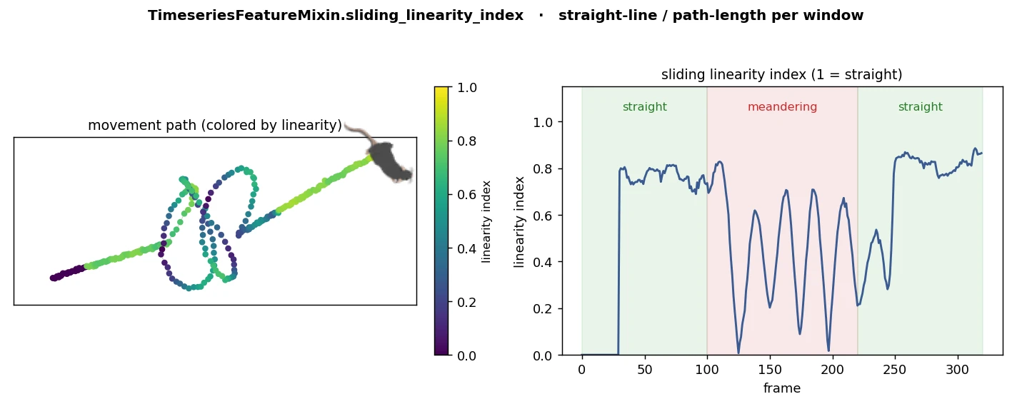
static sliding_linearity_index(x, window_size, sample_rate)[source]

Calculates the Linearity Index (Path Straightness) over a sliding window for a path represented by an array of points.

The Linearity Index measures how straight a path is by comparing the straight-line distance between the start and end points of each window to the total distance traveled along the path.

Parameters

x (np.ndarray) – An (N, M) array representing the path, where N is the number of points and M is the number of spatial dimensions (e.g., 2 for 2D or 3 for 3D). Each row represents the coordinates of a point along the path.
window_size (float) – The size of the sliding window in seconds. This defines the time window over which the linearity index is calculated. The window size should be specified in seconds.
sample_rate (float) – The sample rate in Hz (samples per second), which is used to convert the window size from seconds to frames.

Returns

A 1D array of length N, where each element represents the linearity index of the path within a sliding window. The value is a ratio between the straight-line distance and the actual path length for each window. Values range from 0 to 1, with 1 indicating a perfectly straight path.

Return type

np.ndarray

Example

>>> x = np.random.randint(0, 100, (100, 2))
>>> TimeseriesFeatureMixin.sliding_linearity_index(x=x, window_size=1, sample_rate=10)

static sliding_longest_strike(data, threshold, time_windows, sample_rate, above)[source]

Jitted compute of the length of the longest strike of values within sliding time windows that satisfy a given condition.

Calculates the length of the longest consecutive sequence of values in a 1D NumPy array, where each sequence is determined by a sliding time window. The condition is specified by a threshold, and you can choose whether to look for values above or below the threshold.

Parameters

data (np.ndarray) – The input 1D NumPy array containing the values to be analyzed.
threshold (float) – The threshold value used for the comparison.
time_windows (np.ndarray) – An array containing the time window sizes in seconds.
sample_rate (int) – The sample rate in samples per second.
above (bool) – If True, the function looks for strikes where values are above or equal to the threshold. If False, it looks for strikes where values are below or equal to the threshold.

Return np.ndarray

A 2D NumPy array with dimensions (data.shape[0], time_windows.shape[0]). Each element in the array represents the length of the longest strike that satisfies the condition for the

corresponding time window.

Example

>>> data = np.array([1, 8, 2, 10, 8, 6, 8, 1, 1, 1]).astype(np.float32)
>>> TimeseriesFeatureMixin().sliding_longest_strike(data=data, threshold=7, above=True, time_windows=np.array([1.0]), sample_rate=2)
>>> [[-1.][ 1.][ 1.][ 1.][ 2.][ 1.][ 1.][ 1.][ 0.][ 0.]]
>>> TimeseriesFeatureMixin().sliding_longest_strike(data=data, threshold=7, above=True, time_windows=np.array([1.0]), sample_rate=2)
>>> [[-1.][ 1.][ 1.][ 1.][ 0.][ 1.][ 1.][ 1.][ 2.][ 2.]]

static sliding_mean_squared_jerk(x, window_size, sample_rate)[source]

Calculates the mean squared jerk (rate of change of acceleration) for a position path in a sliding window.

Jerk is the derivative of acceleration, and this function computes the mean squared jerk over sliding windows across the entire path. High jerk values indicate abrupt changes in acceleration, while low values indicate smoother motion.

Parameters

x (np.ndarray) – An (N, M) array representing the path of an object, where N is the number of samples (time steps) and M is the number of spatial dimensions (e.g., 2 for 2D motion). Each row represents the position at a time step.
window_size (float) – The size of each sliding window in seconds. This defines the interval over which the mean squared jerk is calculated.
sample_rate (float) – The sampling rate in Hz (samples per second), which is used to convert the window size from seconds to frames.

Returns

A 1D array of length N, containing the mean squared jerk for each sliding window that ends at each time step. The first frame_step values are set to -1.0, as they do not have enough preceding data points to compute jerk over the full window.

Return type

np.ndarray

Example

>>> x = np.random.randint(0, 500, (12, 2))
>>> TimeseriesFeatureMixin.sliding_mean_squared_jerk(x=x, window_size=1.0, sample_rate=2)

Example II

>>> jerky_path = np.zeros((100, 2))
>>> jerky_path[::10] = np.random.randint(0, 500, (10, 2))
>>> non_jerky_path = np.linspace(0, 500, 100).reshape(-1, 1)
>>> non_jerky_path = np.hstack((non_jerky_path, non_jerky_path))
>>> jerky_jerk_result = TimeseriesFeatureMixin.sliding_mean_squared_jerk(jerky_path, 1.0, 10)
>>> non_jerky_jerk_result = TimeseriesFeatureMixin.sliding_mean_squared_jerk(non_jerky_path, 1.0, 10)

static sliding_momentum_magnitude(x, mass, sample_rate, time_window)[source]

Compute the sliding window momentum magnitude for 2D positional data.

Parameters

x (np.ndarray) – 2D array of shape (n_samples, 2) representing positions.
mass (np.ndarray) – Array of mass values for each frame.
sample_rate (float) – Sampling rate in FPS.
time_window (float) – Time window in seconds for sliding momentum calculation.

Returns

Momentum magnitudes computed for each frame, with results from frames that cannot form a complete window filled with -1.0.

Return type

np.ndarray

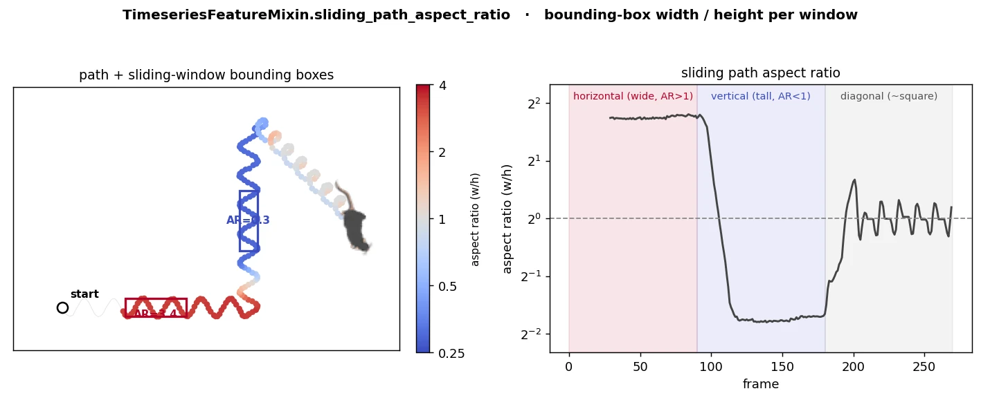
static sliding_path_aspect_ratio(x, window_size, sample_rate, px_per_mm)[source]

Computes the aspect ratio of the bounding box for a sliding window along a path.

This function calculates the aspect ratio (width/height) of the smallest bounding box that encloses a sequence of points within a sliding window over a 2D path. The path is defined by consecutive (x, y) coordinates. The sliding window moves forward by one point at each step, and the aspect ratio is computed for each position of the window.

Parameters

x (np.ndarray) – A 2D array of shape (N, 2) representing the path, where N is the number of points, and each point has two spatial coordinates (x and y).
window_size (float) – The size of the sliding window in seconds.
px_per_mm (float) – Conversion factor representing the number of pixels per millimeter
sample_rate (float) – The sample rate of the path data in points per second.

Returns

An array of aspect ratios for each position of the sliding window. If the window contains a path segment that is aligned vertically or horizontally (leading to a zero width or height), the function returns -1.0 for that position. NaN values are used for the initial positions where the window cannot be fully applied.

Return type

np.ndarray

Example

>>> x = np.random.randint(0, 500, (10, 2))
>>> TimeseriesFeatureMixin.(x=x, window_size=1, sample_rate=2)

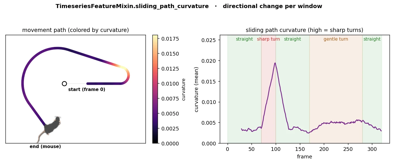
sliding_path_curvature(agg_type, window_size, sample_rate)[source]

Computes the curvature of a path over sliding windows along the path points, providing a measure of the path’s bending or turning within each window.

This function calculates curvature for each window segment by evaluating directional changes. It provides the option to aggregate curvature values within each window using the mean, median, or maximum, depending on the desired level of sensitivity to bends and turns. A higher curvature value indicates a sharper or more frequent directional change within the window, while a lower curvature suggests a straighter or smoother path.

Parameters

x – A 2D array of shape (N, 2) representing the path, where N is the number of points, and each point has two spatial coordinates (e.g., x and y for 2D space).
agg_type (Literal['mean', 'median', 'max']) – Type of aggregation for the curvature within each window.
window_size (float) – Duration of the window in seconds, used to define the size of each segment over which curvature is calculated.
sample_rate (float) – The rate at which path points were sampled (in points per second), used to convert the window size from seconds to frames

Returns

An array of shape (N,) containing the computed curvature values for each window position along the path. Each element represents the aggregated curvature within a specific window, with NaN values for frames where the window does not fit.

Return type

np.ndarray

Example

>>> x = np.random.randint(0, 500, (91, 2))
>>> results = TimeseriesFeatureMixin.sliding_path_curvature(x=x, agg_type='mean', window_size=1, sample_rate=30)

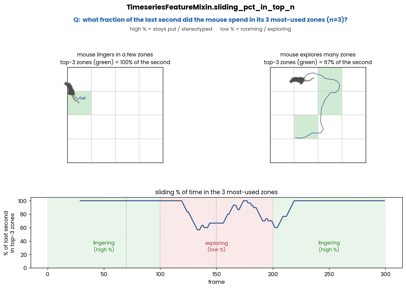
static sliding_pct_in_top_n(x, windows, n, fps)[source]

Compute the percentage of elements in the top ‘n’ frequencies in sliding windows of the input array.

Note

To compute percentage of elements in the top ‘n’ frequencies in entire array, use simba.mixins.statistics_mixin.Statistics.pct_in_top_n().

Parameters

x (np.ndarray) – Input 1D array.
windows (np.ndarray) – Array of window sizes in seconds.
n (int) – Number of top frequencies.
fps (float) – Sampling frequency for time convesrion.

Returns

2D array of computed percentages of elements in the top ‘n’ frequencies for each sliding window.

Return type

np.ndarray

Example

>>> x = np.random.randint(0, 10, (100000,))
>>> results = TimeseriesFeatureMixin.sliding_pct_in_top_n(x=x, windows=np.array([1.0]), n=4, fps=10)

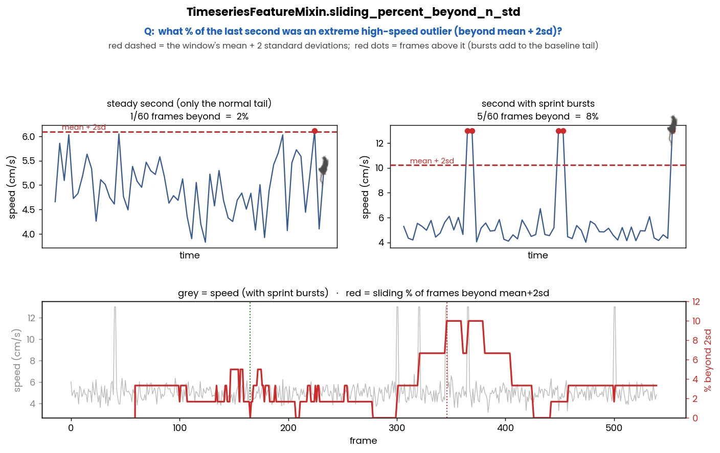
static sliding_percent_beyond_n_std(data, n, window_sizes, sample_rate)[source]

Computed the percentage of data points that exceed ‘n’ standard deviations from the mean for each position in the time series using various window sizes. It returns a 2D array where each row corresponds to a position in the time series, and each column corresponds to a different window size. The results are given as a percentage of data points beyond the threshold.

Parameters

data (np.ndarray) – The input time series data.
n (float) – The number of standard deviations to determine the threshold.
window_sizes (np.ndarray) – An array of window sizes (in seconds) to use for the sliding calculation.
sample_rate (int) – The sampling rate (samples per second) of the time series data.

Returns

A 2D array containing the percentage of data points beyond the specified ‘n’ standard deviations for each window size.

Return type

np.ndarray

static sliding_percent_in_percentile_window(data, upper_pct, lower_pct, window_sizes, sample_rate)[source]

Jitted compute of the percentage of data points falling within a percentile window in a sliding manner.

The function computes the percentage of data points within the specified percentile window for each position in the time series using various window sizes. It returns a 2D array where each row corresponds to a position in the time series, and each column corresponds to a different window size. The results are given as a percentage of data points within the percentile window.

Parameters

data (np.ndarray) – The input time series data.
upper_pct (int) – The upper percentile value for the window (e.g., 95 for the 95th percentile).
lower_pct (int) – The lower percentile value for the window (e.g., 5 for the 5th percentile).
window_sizes (np.ndarray) – An array of window sizes (in seconds) to use for the sliding calculation.
sample_rate (int) – The sampling rate (samples per second) of the time series data.

Returns

A 2D array containing the percentage of data points within the percentile window for each window size.

Return type

np.ndarray

static sliding_percentile_difference(data, upper_pct, lower_pct, window_sizes, fps)[source]

Jitted computes the difference between the upper and lower percentiles within a sliding window for each position in the time series using various window sizes. It returns a 2D array where each row corresponds to a position in the time series, and each column corresponds to a different window size. The results are calculated as the absolute difference between upper and lower percentiles divided by the median of the window.

Parameters

data (np.ndarray) – The input time series data.
upper_pct (int) – The upper percentile value for the window (e.g., 95 for the 95th percentile).
lower_pct (int) – The lower percentile value for the window (e.g., 5 for the 5th percentile).
window_sizes (np.ndarray) – An array of window sizes (in seconds) to use for the sliding calculation.
sample_rate (int) – The sampling rate (samples per second) of the time series data.

Returns

A 2D array containing the difference between upper and lower percentiles for each window size.

Return type

np.ndarray

static sliding_petrosian_fractal_dimension(data, window_sizes, sample_rate)[source]

Jitted compute of Petrosian Fractal Dimension over sliding windows in a data array.

This method computes the Petrosian Fractal Dimension for sliding windows of varying sizes applied to the input data array. The Petrosian Fractal Dimension is a measure of signal complexity.

Note

Adapted from eeglib.

Parameters

data (np.ndarray) – Input data array.
window_sizes (np.ndarray) – Array of window sizes (in seconds).
sample_rate (int) – Sampling rate of the data in samples per second.

Return np.ndarray

An array containing Petrosian Fractal Dimension values for each window size and data point. The shape of the result array is (data.shape[0], window_sizes.shape[0]).

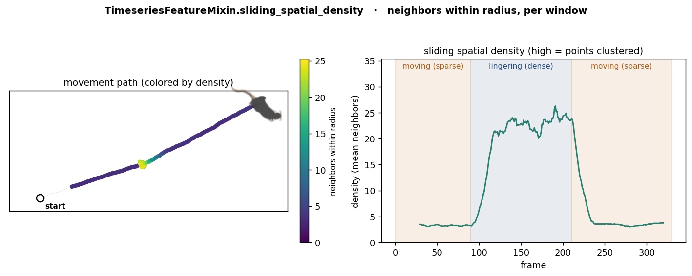
static sliding_spatial_density(x, radius, pixels_per_mm, window_size, sample_rate)[source]

Computes the sliding spatial density of trajectory points in a 2D array, based on the number of neighboring points within a specified radius, considering the density over a moving window of points. This function accounts for the spatial scale in pixels per millimeter, providing a density measurement that is adjusted for the physical scale of the trajectory.

Parameters

x (np.ndarray) – A 2D array of shape (N, 2), where N is the number of points and each point has two spatial coordinates (x, y). The array represents the trajectory path of points in a 2D space (e.g., x and y positions in space).
radius (float) – The radius (in millimeters) within which to count neighboring points around each trajectory point. Defines the area of interest around each point.
pixels_per_mm (float) – The scaling factor that converts the physical radius (in millimeters) to pixel units for spatial density calculations.
window_size (float) – The size of the sliding window (in seconds or points) to compute the density of points. A larger window size will consider more points in each density calculation.
sample_rate (float) – The rate at which to sample the trajectory points (e.g., frames per second or samples per unit time). It adjusts the granularity of the sliding window.

Returns

A 1D numpy array where each element represents the computed spatial density for the trajectory at the corresponding point in time (or frame). Higher values indicate more densely packed points within the specified radius, while lower values suggest more sparsely distributed points.

Return type

np.ndarray

Example

>>> x = np.random.randint(0, 20, (100, 2))  # Example trajectory with 100 points in 2D space
>>> results = TimeseriesFeatureMixin.sliding_spatial_density(x=x, radius=5.0, pixels_per_mm=10.0, window_size=1, sample_rate=31)

static sliding_stationary(data, time_windows, sample_rate, test='adf')[source]

Perform the Augmented Dickey-Fuller (ADF), Kwiatkowski-Phillips-Schmidt-Shin (KPSS), or Zivot-Andrews test on sliding windows of time series data. Parallel processing using all available cores is used to accelerate computation.

Note

ADF: A high p-value suggests non-stationarity, while a low p-value indicates stationarity.
KPSS: A high p-value suggests stationarity, while a low p-value indicates non-stationarity.
ZA: A high p-value suggests non-stationarity, while a low p-value indicates stationarity.

Parameters

data (np.ndarray) – 1-D NumPy array containing the time series data to be tested.
time_windows (np.ndarray) – A 1-D NumPy array containing the time window sizes in seconds.
sample_rate (np.ndarray) – The sample rate of the time series data (samples per second).
test (Literal) – Test to perfrom: Options: ‘ADF’ (Augmented Dickey-Fuller), ‘KPSS’ (Kwiatkowski-Phillips-Schmidt-Shin), ‘ZA’ (Zivot-Andrews).

Returns

A tuple of two 2-D NumPy arrays containing test statistics and p-values. - The first array (stat) contains the ADF test statistics. - The second array (p_vals) contains the corresponding p-values

Return type

Tuple[np.ndarray, np.ndarray]

Example

>>> data = np.array([1, 2, 3, 4, 5, 6, 7, 8, 9, 10])
>>> TimeseriesFeatureMixin().sliding_stationary(data=data, time_windows=np.array([2.0]), test='KPSS', sample_rate=2)

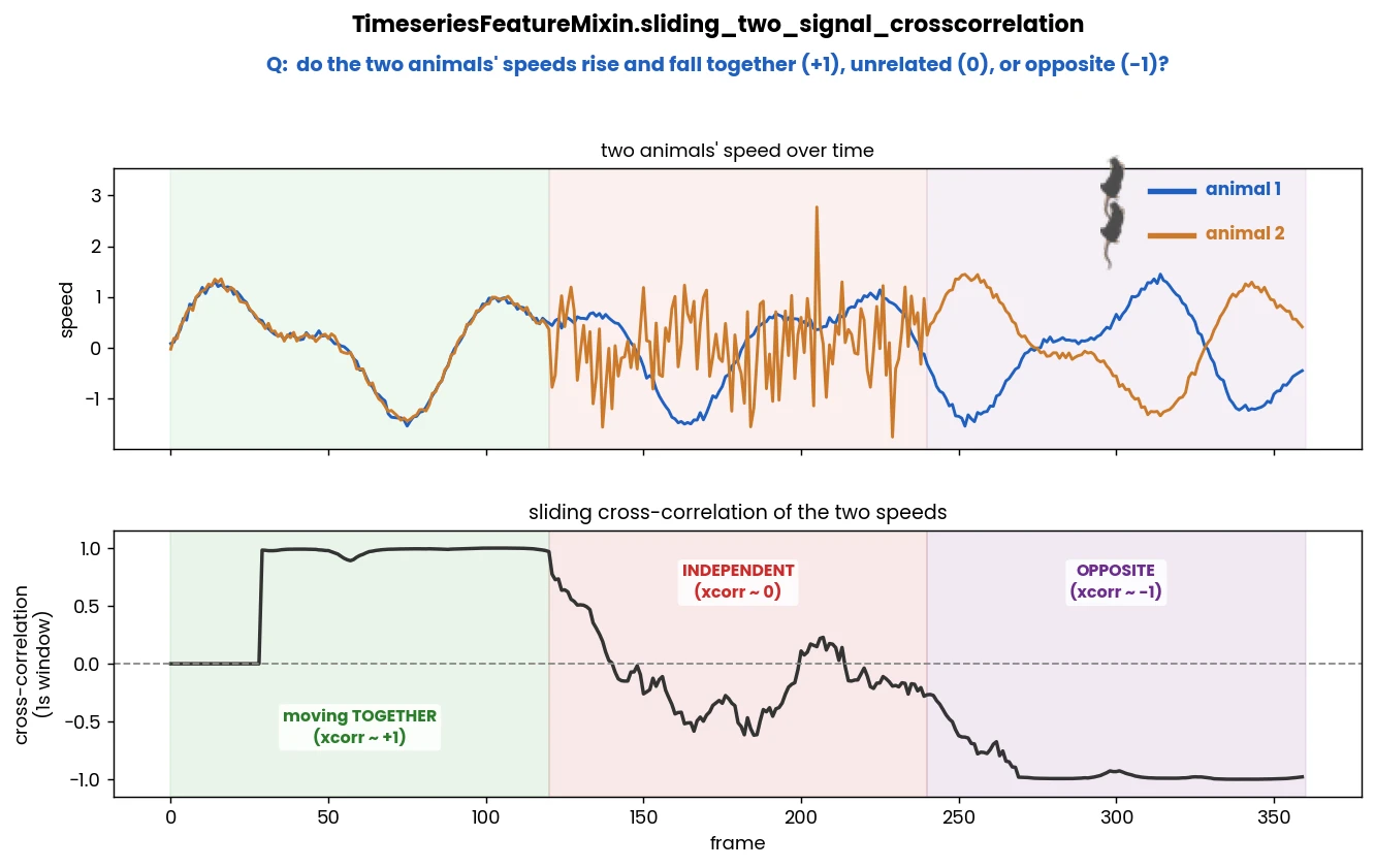
static sliding_two_signal_crosscorrelation(x, y, windows, sample_rate, normalize, lag)[source]

Calculate sliding (lagged) cross-correlation between two signals, e.g., the movement and velocity of two animals.

Note

If no lag needed, pass lag 0.0.

Parameters

x (np.ndarray) – The first input signal.
y (np.ndarray) – The second input signal.
windows (np.ndarray) – Array of window lengths in seconds.
sample_rate (float) – Sampling rate of the signals (in Hz or FPS).
normalize (bool) – If True, normalize the signals before computing the correlation.
lag (float) – Time lag between the signals in seconds.

Returns

2D array of sliding cross-correlation values. Each row corresponds to a time index, and each column corresponds to a window size specified in the windows parameter.

Return type

np.ndarray

Example

>>> x = np.random.randint(0, 10, size=(20,))
>>> y = np.random.randint(0, 10, size=(20,))
>>> TimeseriesFeatureMixin.sliding_two_signal_crosscorrelation(x=x, y=y, windows=np.array([1.0, 1.2]), sample_rate=10, normalize=True, lag=0.0)

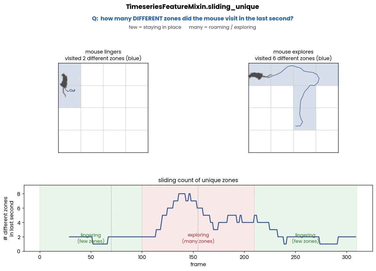
static sliding_unique(x, time_windows, fps)[source]

Compute the number of unique values in a sliding window over an array of feature values.

Parameters

x – 1D array of feature values for which the unique values are to be counted.
time_windows – Array of window sizes (in seconds) for which the unique values are counted.
fps (int) – The frame rate in frames per second, which is used to calculate the window size in samples.

Returns

A 2D array where each row corresponds to a time window, and each element represents the count of unique values in the corresponding sliding window of the array x.

Return type

np.ndarray

static sliding_variance(data, window_sizes, sample_rate)[source]

Jitted compute of the variance of data within sliding windows of varying sizes applied to the input data array. Variance is a measure of data dispersion or spread.

Parameters

data – 1d input data array.
window_sizes – Array of window sizes (in seconds).
sample_rate – Sampling rate of the data in samples per second.

Returns

Variance values for each window size and data point. The shape of the result array is (data.shape[0], window_sizes.shape[0]).

Example

>>> data = np.array([1, 2, 3, 1, 2, 9, 17, 2, 10, 4]).astype(np.float32)
>>> TimeseriesFeatureMixin().sliding_variance(data=data, window_sizes=np.array([0.5]), sample_rate=10)
>>> [[-1.],[-1.],[-1.],[-1.],[ 0.56],[ 8.23],[35.84],[39.20],[34.15],[30.15]])

static sliding_window_stats(data, window_sizes, sample_rate, statistics)[source]

Compute descriptive statistics over sliding windows in 1D data array.

This function is a wrapper around TimeseriesFeatureMixin.sliding_descriptive_statistics that provides input validation and preprocessing. It computes various descriptive statistics for sliding windows of varying sizes applied to the input data array.

Note

Validation wrapper for `func:`simba.mixins.timeseries_features_mixin.TimeseriesFeatureMixin.sliding_descriptive_statistics

Parameters

data (np.ndarray) – 1D input data array containing the time series values to analyze.
window_sizes (Union[List, np.ndarray]) – Array or list of window sizes (in seconds) for computing statistics.
sample_rate (float) – Sampling rate of the data in samples per second (e.g., fps for video data).
statistics (List[Literal["var", "max", "min", "std", "median", "mean", "mad", "sum", "mac", "rms", "absenergy"]]) – List of statistics to compute. Available options: - ‘var’: variance - ‘max’: maximum value - ‘min’: minimum value - ‘std’: standard deviation - ‘median’: median value - ‘mean’: mean value - ‘mad’: median absolute deviation - ‘sum’: sum of values - ‘mac’: mean absolute change - ‘rms’: root mean square - ‘absenergy’: absolute energy

Return np.ndarray

Array containing the selected descriptive statistics for each window size, data point, and statistic type. Shape is (len(statistics), data.shape[0], window_sizes.shape[0]).

Return type

np.ndarray

Example

>>> data = np.array([1.0, 4.0, 2.0, 3.0, 5.0, 6.0, 8.0, 7.0, 9.0, 10.0]).astype(np.float32)
>>> window_sizes = [0.5, 1.0, 1.5, 2.0]
>>> sample_rate = 30.0  # 30 fps
>>> statistics = ['mean', 'std', 'max']
>>> results = sliding_window_stats(data=data, window_sizes=window_sizes, sample_rate=sample_rate, statistics=statistics)

static spatial_density(x, radius, pixels_per_mm)[source]

Computes the spatial density of trajectory points in a 2D array, based on the number of neighboring points within a specified radius for each point in the trajectory.

Spatial density provides insights into the movement pattern along a trajectory. Higher density values indicate areas where points are closely packed, which can suggest slower movement, lingering, or frequent changes in direction. Lower density values suggest more spread-out points, often associated with faster, more linear movement.

The function calculates spatial density by counting the number of points within a specified radius around each trajectory point and averaging these counts across all points.

Radius: The radius specifies the neighborhood around each point, within which other points are counted as neighbors.
Pixels per mm: This parameter scales the radius from physical units (e.g., millimeters) to pixel units, making the method adaptable to different spatial scales.

Parameters

x (np.ndarray) – A 2D array of shape (N, 2), where N is the number of points and each point has two spatial coordinates.
radius (float) – The radius within which to count neighboring points around each point. Defines the area of interest around each trajectory point.

Returns

A single float value representing the average spatial density of the trajectory.

Return type

float

Example

>>> x = np.array([[0, 0], [1, 1], [2, 2], [3, 3], [4, 4], [1, 0.5], [1.5, 1.5]])
>>> density = TimeseriesFeatureMixin.spatial_density(x, pixels_per_mm=2.5, radius=5)
>>> high_density_points = np.array([[0, 0], [0.5, 0], [1, 0], [1.5, 0], [2, 0], [0, 0.5], [0.5, 0.5], [1, 0.5], [1.5, 0.5], [2, 0.5]])
>>> low_density_points = np.array([[0, 0], [5, 5], [10, 10], [15, 15], [20, 20]])
>>> high = TimeseriesFeatureMixin.spatial_density(x=high_density_points,radius=1, pixels_per_mm=1)
>>> low = TimeseriesFeatureMixin.spatial_density(x=low_density_points,radius=1, pixels_per_mm=1)

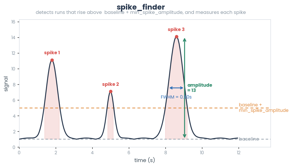
static spike_finder(data, sample_rate, baseline, min_spike_amplitude, min_fwhm=- inf, min_half_width=- inf)[source]

Identify and characterize spikes in a given time-series data sequence. This method identifies spikes in the input data based on the specified criteria and characterizes each detected spike by computing its amplitude, full-width at half maximum (FWHM), and half-width.

Parameters

data (np.ndarray) – A 1D array containing the input data sequence to analyze.
sample_rate (int) – The sample rate, indicating how many data points are collected per second.
baseline (float) – The baseline value used to identify spikes. Any data point above (baseline + min_spike_amplitude) is considered part of a spike.
min_spike_amplitude (float) – The minimum amplitude (above baseline) required for a spike to be considered.
min_fwhm (Optional[float]) – The minimum full-width at half maximum (FWHM) for a spike to be included. If not specified, it defaults to negative infinity, meaning it is not considered for filtering.
min_half_width (Optional[float]) – The minimum half-width required for a spike to be included. If not specified, it defaults to negative infinity, meaning it is not considered for filtering.

Return tuple

A tuple containing three elements: - spike_idx (List[np.ndarray]): A list of 1D arrays, each representing the indices of the data points belonging to a detected spike. - spike_vals (List[np.ndarray]): A list of 1D arrays, each containing the values of the data points within a detected spike. - spike_dict (Dict[int, Dict[str, float]]): A dictionary where the keys are spike indices, and the values are dictionaries containing spike characteristics including ‘amplitude’ (spike amplitude), ‘fwhm’ (FWHM), and ‘half_width’ (half-width).

Note

The function uses the Numba JIT (Just-In-Time) compilation for optimized performance. Without fastmath=True there is no runtime improvement over standard numpy.

Example

>>> data = np.array([0.1, 0.1, 0.3, 0.1, 10, 10, 8, 0.1, 0.1, 0.1, 10, 10, 8, 99, 0.1, 99, 99, 0.1]).astype(np.float32)
>>> spike_idx, spike_vals, spike_stats = TimeseriesFeatureMixin().spike_finder(data=data, baseline=1, min_spike_amplitude=5, sample_rate=2, min_fwhm=-np.inf, min_half_width=0.0002)

static spike_train_finder(data, spike_idx, sample_rate, min_spike_train_length=inf, max_spike_train_separation=inf)[source]

Identify and analyze spike trains from a list of spike indices.

This function takes spike indices and additional information, such as the data, sample rate, minimum spike train length, and maximum spike train separation, to identify and analyze spike trains in the data.

Note

The function may return an empty dictionary if no spike trains meet the criteria.
A required input is spike_idx, which is returned by spike_finder().

Parameters

data (np.ndarray) – The data from which spike trains are extracted.
spike_idx (types.List(types.Array(types.int64, 1, 'C'))) – A list of spike indices, typically as integer timestamps.
sample_rate (float) – The sample rate of the data.
min_spike_train_length (Optional[float]) – The minimum length a spike train must have to be considered. Default is set to positive infinity, meaning no minimum length is enforced.
max_spike_train_separation (Optional[float]) – The maximum allowable separation between spikes in the same train. Default is set to positive infinity, meaning no maximum separation is enforced.

Return DictType[int64,DictType[unicode_type,float64]]

A dictionary containing information about identified spike trains.

Each entry in the returned dictionary is indexed by an integer, and contains the following information:

‘train_start_time’: Start time of the spike train in seconds.
‘train_end_time’: End time of the spike train in seconds.
‘train_start_obs’: Start time index in observations.
‘train_end_obs’: End time index in observations.
‘spike_cnt’: Number of spikes in the spike train.
‘train_length_obs_cnt’: Length of the spike train in observations.
‘train_length_obs_s’: Length of the spike train in seconds.
‘train_spike_mean_lengths_s’: Mean length of individual spikes in seconds.
‘train_spike_std_length_obs’: Standard deviation of spike lengths in observations.
‘train_spike_std_length_s’: Standard deviation of spike lengths in seconds.
‘train_spike_max_length_obs’: Maximum spike length in observations.
‘train_spike_max_length_s’: Maximum spike length in seconds.
‘train_spike_min_length_obs’: Minimum spike length in observations.
‘train_spike_min_length_s’: Minimum spike length in seconds.
‘train_mean_amplitude’: Mean amplitude of the spike train.
‘train_std_amplitude’: Standard deviation of spike amplitudes.
‘train_min_amplitude’: Minimum spike amplitude.
‘train_max_amplitude’: Maximum spike amplitude.

Example

>>> data = np.array([0.1, 0.1, 0.3, 0.1, 10, 10, 8, 0.1, 0.1, 0.1, 10, 10, 8, 99, 0.1, 99, 99, 0.1]).astype(np.float32)
>>> spike_idx, _, _ = TimeseriesFeatureMixin().spike_finder(data=data, baseline=0.3, min_spike_amplitude=0.2, sample_rate=2, min_fwhm=-np.inf, min_half_width=-np.inf)
>>> results = TimeseriesFeatureMixin().spike_train_finder(data=data, spike_idx=typed.List(spike_idx), sample_rate=2.0, min_spike_train_length=2.0, max_spike_train_separation=2.0)

static time_since_previous_target_value(data, value, fps, inverse=False)[source]

Calculate the time duration (in seconds) since the previous occurrence of a specific value in a data array.

Calculates the time duration, in seconds, between each data point and the previous occurrence of a specific value within the data array.

Parameters

data (np.ndarray) – The input 1D array containing the time series data.
value (float) – The specific value to search for in the data array.
sample_rate (int) – The sampling rate which data points were collected. It is used to calculate the time duration in seconds.
inverse (bool) – If True, the function calculates the time since the previous value that is NOT equal to the specified ‘value’. If False, it calculates the time since the previous occurrence of the specified ‘value’.

Returns

A 1D NumPy array containing the time duration (in seconds) since the previous occurrence of the specified ‘value’ for each data point.

Return type

np.ndarray

Example

>>> data = np.array([8, 8, 2, 10, 8, 6, 8, 1, 1, 1]).astype(np.float32)
>>> TimeseriesFeatureMixin().time_since_previous_target_value(data=data, value=8.0, inverse=False, sample_rate=2.0)
>>> [0. , 0. , 0.5, 1. , 0. , 0.5, 0. , 0.5, 1. , 1.5])
>>> TimeseriesFeatureMixin().time_since_previous_target_value(data=data, value=8.0, inverse=True, sample_rate=2.0)
>>> [-1. , -1. ,  0. ,  0. ,  0.5,  0. ,  0.5,  0. ,  0. ,  0. ]

static time_since_previous_threshold(data, threshold, fps, above)[source]

Jitted compute of the time (in seconds) that has elapsed since the last occurrence of a value above (or below) a specified threshold in a time series. The time series is assumed to have a constant sample rate.

Parameters

data (np.ndarray) – The input 1D array containing the time series data.
threshold (int) – The threshold value used for the comparison.
fps (int) – The sample rate of the time series in samples per second.
above (bool) – If True, the function looks for values above or equal to the threshold. If False, it looks for values below or equal to the threshold.

Return np.ndarray

A 1D array of the same length as the input data. Each element represents the time elapsed (in seconds) since the last occurrence of the threshold value. If no threshold value is found before the current data point, the corresponding result is set to -1.0.

Examples

>>> data = np.array([1, 8, 2, 10, 8, 6, 8, 1, 1, 1]).astype(np.float32)
>>> TimeseriesFeatureMixin().time_since_previous_threshold(data=data, threshold=7.0, above=True, sample_rate=2.0)
>>> [-1. ,  0. ,  0.5,  0. ,  0. ,  0.5,  0. ,  0.5,  1. ,  1.5]
>>> TimeseriesFeatureMixin().time_since_previous_threshold(data=data, threshold=7.0, above=False, sample_rate=2.0)
>>> [0. , 0.5, 0. , 0.5, 1. , 0. , 0.5, 0. , 0. , 0. ]

Time-series statistics GPU methods

simba.data_processors.cuda.timeseries.sliding_hjort_parameters_gpu(data, window_sizes, sample_rate)[source]

Compute Hjorth parameters over sliding windows on the GPU.

See also

For CPU implementation, see :simba.mixins.timeseries_features_mixin.TimeseriesFeatureMixin.hjort_parameters

Parameters

data (np.ndarray) – 1D numeric array of signal data.
window_sizes (np.ndarray) – 1D numeric array of window sizes (in seconds).
sample_rate (int) – Sampling rate of the data (samples per second).

Returns

3D array of shape (3, len(data), len(window_sizes)) containing Hjorth parameters computed for each data point and window size.

Return type

np.ndarray

Example

>>> x = np.random.randint(0, 500, (10,)).astype(np.float32)
>>> window_sizes = np.array([1.0, 0.5]).astype(np.float64)
>>> sample_rate = 10
>>> H = sliding_hjort_parameters_gpu(data=x, window_sizes=window_sizes, sample_rate=sample_rate)

simba.data_processors.cuda.timeseries.sliding_linearity_index_cuda(x, window_size, sample_rate)[source]

Calculates the straightness (linearity) index of a path using CUDA acceleration.

The output is a value between 0 and 1, where 1 indicates a perfectly straight path.

EXPECTED RUNTIMES
FRAMES (MILLIONS)	GPU TIME (S)	GPU TIME (STEV)
2	0.03031	0.002
4	0.05208	0.004
8	0.08882	0.0056
16	0.17612	0.0108
32	0.37699	0.01587
64	0.70194	0.01848
128	1.36778	0.06145
256	3.09965	0.21796
512	17.9707	10.5061
NVIDIA GeForce RTX 4070
time window = 2.5s @ 30 FPS
3 ITERATIONS

Parameters

x (np.ndarray) – An (N, M) array representing the path, where N is the number of points and M is the number of spatial dimensions (e.g., 2 for 2D or 3 for 3D). Each row represents the coordinates of a point along the path.
window_size (float) – The size of the sliding window in seconds. This defines the time window over which the linearity index is calculated. The window size should be specified in seconds.
sample_rate (float) – The sample rate in Hz (samples per second), which is used to convert the window size from seconds to frames.

Returns

A 1D array of length N, where each element represents the linearity index of the path within a sliding window. The value is a ratio between the straight-line distance and the actual path length for each window. Values range from 0 to 1, with 1 indicating a perfectly straight path.

Return type

np.ndarray

Example

>>> x = np.random.randint(0, 500, (100, 2)).astype(np.float32)
>>> q = sliding_linearity_index_cuda(x=x, window_size=2, sample_rate=30)

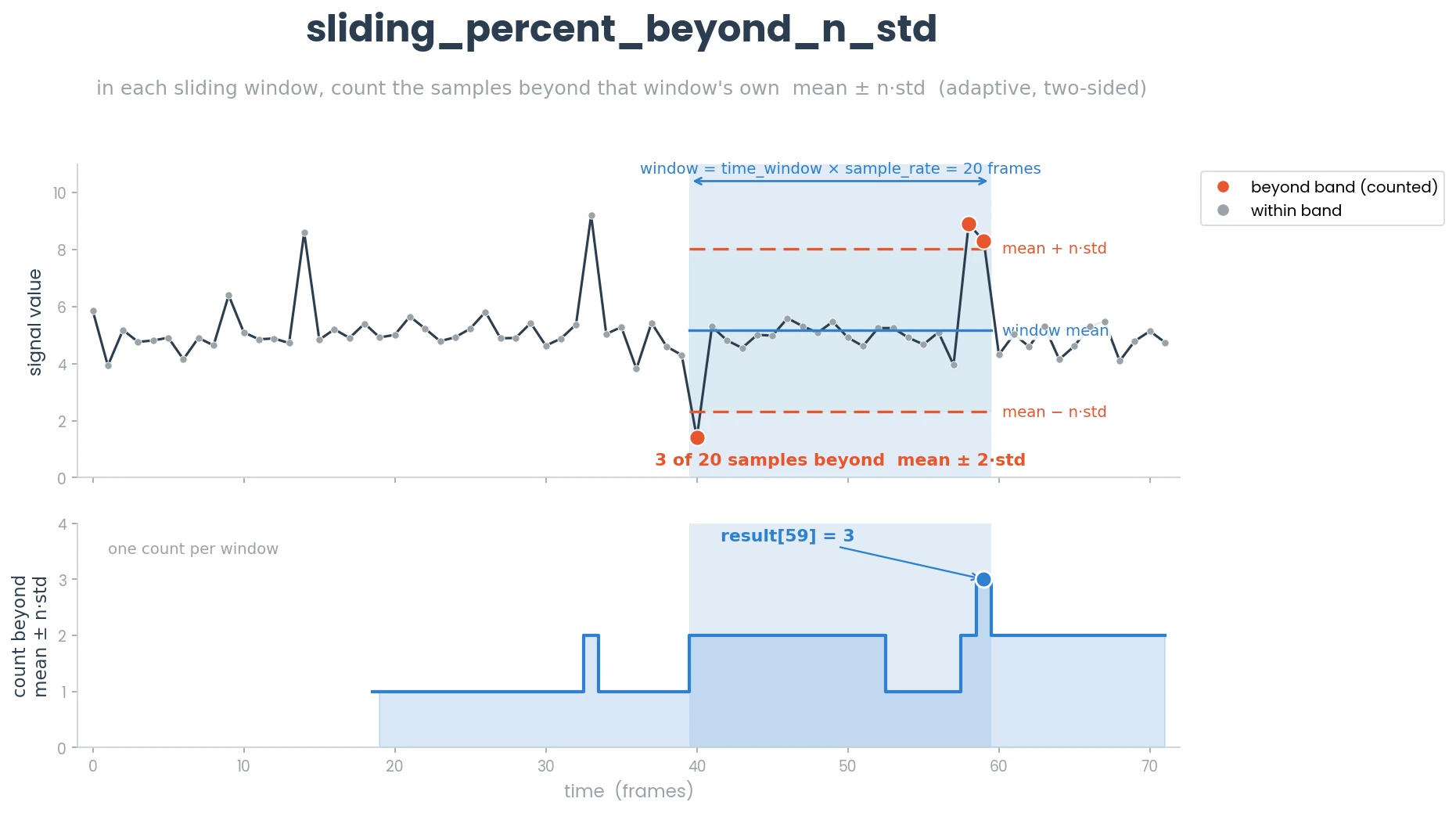
simba.data_processors.cuda.timeseries.sliding_percent_beyond_n_std(data, time_window, sample_rate, value)[source]

Computes the percentage of points in each sliding window of data that fall beyond n standard deviations from the mean of that window.

This function uses GPU acceleration via CUDA to efficiently compute the result over large datasets.

Parameters

data (np.ndarray) – The input 1D data array for which the sliding window computation is to be performed.
time_window (float) – The length of the time window in seconds.
sample_rate (float) – The sample rate of the data in Hz (samples per second).
value (float) – The number of standard deviations beyond which to count data points.

Returns

An array containing the count of data points beyond n standard deviations for each window.

Return type

np.ndarray

Example

>>> data = np.random.randint(0, 100, (100,))
>>> results = sliding_percent_beyond_n_std(data=data, time_window=1, sample_rate=10, value=2)

simba.data_processors.cuda.timeseries.sliding_spatial_density_cuda(x, radius, pixels_per_mm, window_size, sample_rate)[source]

Computes the spatial density of points within a moving window along a trajectory using CUDA for acceleration.

This function calculates a spatial density measure for each point along a 2D trajectory path by counting the number of neighboring points within a specified radius. The computation is performed within a sliding window that moves along the trajectory, using GPU acceleration to handle large datasets efficiently.

EXPECTED RUNTIMES
FRAMES (MILLIONS)	GPU TIME (S)	GPU TIME (STEV)
2	0.5252	0.00063
4	1.0396	0.00099
8	2.0821	0.00231
16	4.2678	0.070249
32	8.4416	0.121225
64	16.941	0.097708
128	34.092	0.03986
256	68.052	0.27862
512	138.78118	3.755006
NVIDIA GeForce RTX 4070
time window = 2.5s @ 30 FPS
3 ITERATIONS

Parameters

x (np.ndarray) – A 2D array of shape (N, 2), where N is the number of points and each point has two spatial coordinates (x, y). The array represents the trajectory path of points in a 2D space (e.g., x and y positions in space).
radius (float) – The radius (in millimeters) within which to count neighboring points around each trajectory point. Defines the area of interest around each point.
pixels_per_mm (float) – The scaling factor that converts the physical radius (in millimeters) to pixel units for spatial density calculations.
window_size (float) – The size of the sliding window (in seconds or points) to compute the density of points. A larger window size will consider more points in each density calculation.
sample_rate (float) – The rate at which to sample the trajectory points (e.g., frames per second or samples per unit time). It adjusts the granularity of the sliding window.

Returns

A 1D numpy array where each element represents the computed spatial density for the trajectory at the corresponding point in time (or frame). Higher values indicate more densely packed points within the specified radius, while lower values suggest more sparsely distributed points.

Return type

np.ndarray

Example

>>> df = pd.read_csv("/mnt/c/troubleshooting/two_black_animals_14bp/project_folder/csv/outlier_corrected_movement_location/Test_3.csv")
>>> x = df[['Nose_1_x', 'Nose_1_y']].values
>>> results_cuda = sliding_spatial_density_cuda(x=x, radius=10.0, pixels_per_mm=4.0, window_size=1, sample_rate=20)

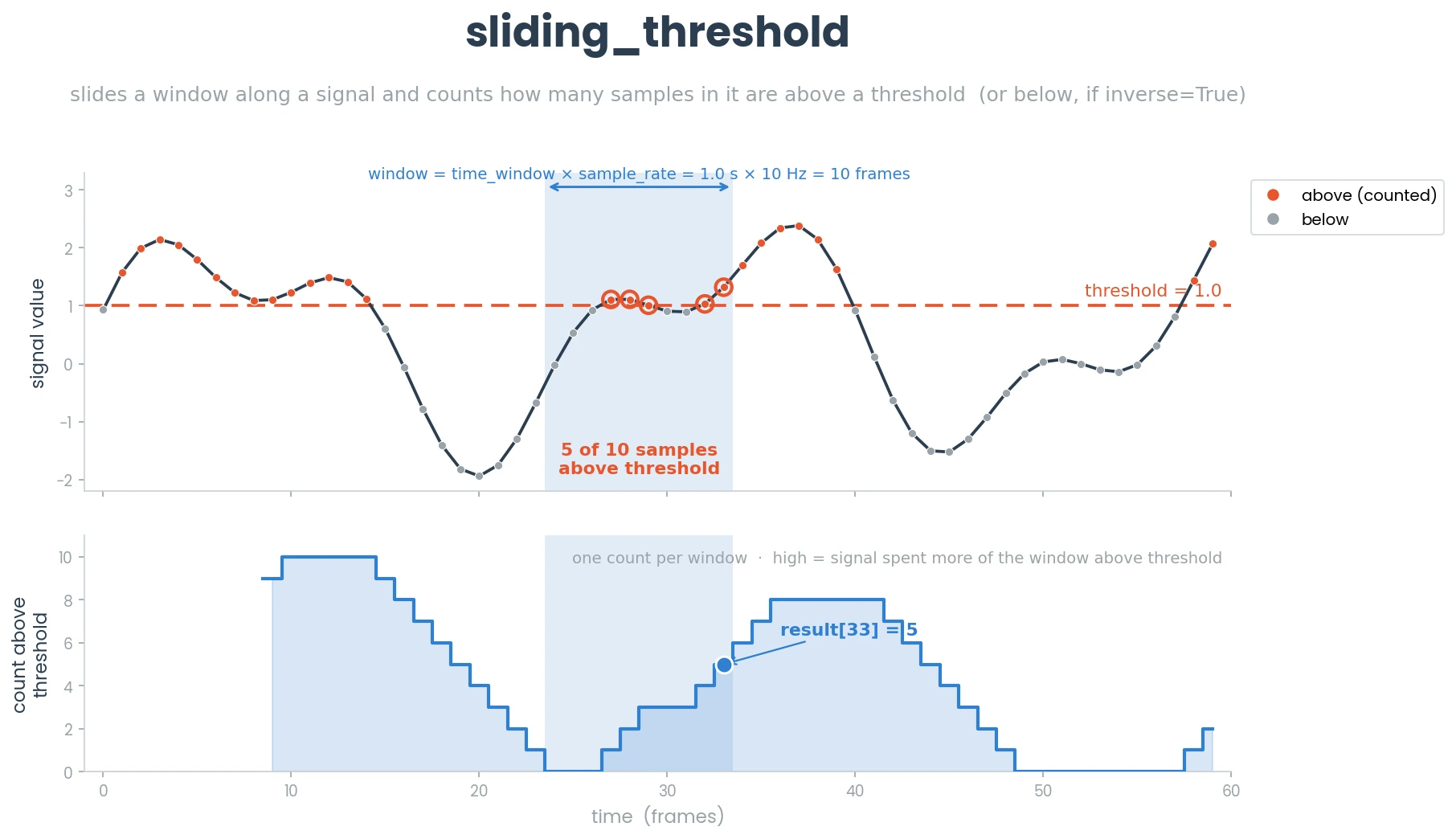
simba.data_processors.cuda.timeseries.sliding_threshold(data, time_window, sample_rate, value, inverse=False)[source]

Compute the count of observations above or below threshold crossings over a sliding window using GPU acceleration.

Parameters

data (np.ndarray) – Input data array.
time_window (float) – Size of the sliding window in seconds.
sample_rate (float) – Number of samples per second in the data.
value (float) – Threshold value.
inverse (Optional[bool]) – If False, counts values above the threshold. If True, counts values below.

Returns

Array containing count of threshold crossings per window.

Return type

np.ndarray