GPU acceleration

SimBA ships CUDA/CuPy-accelerated implementations of many of its most compute-heavy routines — geometry, image, statistics, circular-statistics, time-series and SHAP operations. On a supported NVIDIA GPU these run the same analyses as their CPU counterparts, but orders of magnitude faster on large datasets.

This page is a single consolidated view of every GPU-accelerated module. Each block is also documented in its topical section (e.g. Geometry, Statistics); the canonical, cross-referenceable entries live there, so the listings here mirror them for a one-stop GPU reference.

Geometry (GPU)

simba.data_processors.cuda.geometry.directionality_to_nonstatic_target(left_ear, right_ear, nose, target, verbose=False)

GPU method to calculate if an animal is directing towards a moving point location given the target location and the left ear, right ear, and nose coordinates of the observer.

EXPECTED RUNTIMES
Observations Frames	Mean (s)	Std (s)	Min (s)	Max (s)
10,000	0.147	0.2064	0.0008	0.4389
100,000	0.0056	0.0005	0.0052	0.0063
1,000,000	0.0438	0.0235	0.0239	0.0768
10,000,000	0.2133	0.0046	0.2083	0.2195
50,000,000	1.5716	0.2608	1.2548	1.8936
NVIDIA GeForce RTX 4070
3 ITERATIONS

See also

Input left ear, right ear, and nose coordinates of the observer is returned by simba.mixins.feature_extraction_mixin.FeatureExtractionMixin.check_directionality_viable()

For non-GPU numba based CPU method, see simba.mixins.feature_extraction_mixin.FeatureExtractionMixin.jitted_line_crosses_to_nonstatic_targets()

If the target is static, consider simba.mixins.feature_extraction_mixin.FeatureExtractionMixin.jitted_line_crosses_to_static_targets() or simba.data_processors.cuda.geometry.directionality_to_static_targets() for GPU acceleration.

Parameters

• left_ear (np.ndarray) – 2D array of size len(frames) x 2 with the coordinates of the observer animals left ear

• right_ear (np.ndarray) – 2D array of size len(frames) x 2 with the coordinates of the observer animals right ear

• nose (np.ndarray) – 2D array of size len(frames) x 2 with the coordinates of the observer animals nose

• target (np.ndarray) – 1D array of with x,y of target location

Returns

2D array of size len(frames) x 4. First column represent the side of the observer that the target is in view. 0 = Left side, 1 = Right side, 2 = Not in view. Second and third column represent the x and y location of the observer animals eye (half-way between the ear and the nose). Fourth column represent if target is view (bool).

Return type

np.ndarray

Example

>>> left_ear = np.random.randint(0, 500, (100, 2))
>>> right_ear = np.random.randint(0, 500, (100, 2))
>>> nose = np.random.randint(0, 500, (100, 2))
>>> target = np.random.randint(0, 500, (100, 2))
>>> directionality_to_nonstatic_target(left_ear=left_ear, right_ear=right_ear, nose=nose, target=target)

simba.data_processors.cuda.geometry.directionality_to_static_targets(left_ear, right_ear, nose, target, verbose=False)

GPU helper to calculate if an animal is directing towards a static location (e.g., ROI centroid), given the target location and the left ear, right ear, and nose coordinates of the observer.

Note

Input left ear, right ear, and nose coordinates of the observer is returned by simba.mixins.feature_extraction_mixin.FeatureExtractionMixin.check_directionality_viable()

See also

For numba based CPU method, see simba.mixins.feature_extraction_mixin.FeatureExtractionMixin.jitted_line_crosses_to_static_targets() If the target is moving, consider simba.mixins.feature_extraction_mixin.FeatureExtractionMixin.jitted_line_crosses_to_nonstatic_targets().

EXPECTED RUNTIMES
FRAMES (MILLIONS)	GPU TIME (S)	GPU TIME (STEV)
10	0.1005	0.02
20	0.1918	0.04
40	0.4382	0.094
80	0.912	0.2904
160	2.8023	1.2692
240	5.7812	3.85148
NVIDIA GeForce RTX 4070
3 ITERATIONS

Parameters

• left_ear (np.ndarray) – 2D array of size len(frames) x 2 with the coordinates of the observer animals left ear

• right_ear (np.ndarray) – 2D array of size len(frames) x 2 with the coordinates of the observer animals right ear

• nose (np.ndarray) – 2D array of size len(frames) x 2 with the coordinates of the observer animals nose

• target (np.ndarray) – 1D array of with x,y of target location

Returns

2D array of size len(frames) x 4. First column represent the side of the observer that the target is in view. 0 = Left side, 1 = Right side, 2 = Not in view. Second and third column represent the x and y location of the observer animals eye (half-way between the ear and the nose). Fourth column represent if target is view (bool).

Return type

np.ndarray

Example

>>> left_ear = np.random.randint(0, 500, (100, 2))
>>> right_ear = np.random.randint(0, 500, (100, 2))
>>> nose = np.random.randint(0, 500, (100, 2))
>>> target = np.random.randint(0, 500, (2))
>>> directionality_to_static_targets(left_ear=left_ear, right_ear=right_ear, nose=nose, target=target)

simba.data_processors.cuda.geometry.find_midpoints(x, y, percentile=0.5, batch_size=15000000)

Calculate the midpoints between corresponding points in arrays x and y based on a given percentile using GPU acceleration.

For example, calculate the midpoint between the animal ears (to get presumed nape) or lateral sides (to get presumed center of mass), or nose and left ear (to get left eye) etc.

This function computes the midpoints between each pair of points (x[i], y[i]) from the input arrays x and y. The midpoint is calculated by taking a weighted sum of the differences along each axis, where the weight is determined by the specified percentile. The computation is performed in batches to handle large datasets efficiently.

See also

For CPU function see simba.mixins.feature_extraction_mixin.FeatureExtractionMixin.find_midpoints().

EXPECTED RUNTIMES
OBSERVATIONS (MILLIONS)	TIME (S)	STD (S)
2	0.014	0.004
4	0.022	0.015
8	0.039	0.025
16	0.073	0.057
32	0.161	0.102
64	0.290	0.205
128	0.609	0.477
512	2.100	0.9

Parameters

• x (np.ndarray) – An array of shape (n, 2) representing the x-coordinates of n points.

• y (np.ndarray) – An array of shape (n, 2) representing the y-coordinates of n points.

• percentile – A float value between 0 and 1 indicating the percentile to use when calculating the midpoints. The default value is 0.5, which corresponds to the middle.

• batch_size (Optional[int]) – An integer specifying the batch size for processing the input arrays. Larger batch sizes will use more memory but may be faster. The default value is 15 million (1.5e+7).

Returns

An array of shape (n, 2) containing the calculated midpoints for each pair of corresponding points in x and y.

Return type

np.ndarray

Example

>>> x = np.random.randint(0, 100, (100, 2)).astype(np.int8)
>>> y = np.random.randint(0, 100, (100, 2)).astype(np.int8)
>>> p = find_midpoints(x=x, y=y)

simba.data_processors.cuda.geometry.get_convex_hull(pts)

Compute the convex hull for each set of 2D points in parallel using CUDA and the Jarvis March algorithm. This function processes a batch of 2D point sets (frames) and computes the convex hull for each set. The convex hull of a set of points is the smallest convex polygon that contains all the points.

The function uses a variant of the Gift Wrapping algorithm (Jarvis March) to compute the convex hull. It finds the leftmost point, then iteratively determines the next point on the hull by checking the orientation of the remaining points. The results are stored in the results array, where each row corresponds to a frame and contains the indices of the points forming the convex hull. Points not on the hull are marked with -1.

EXPECTED RUNTIMES
FRAMES	TIME (S)
110k	0.009
181k	0.014
327k	0.026
620k	0.049
1.2m	0.095
2.4m	0.18
4.7m	0.351
9m	0.865
17.9m	1.452
35.8m	5.695
71.6m	7.243
NVIDIA GeForce RTX 4070
7 body-parts

Note

Implements the Jarvis March (gift-wrapping) convex-hull algorithm (Jarvis, R. A., 1973, Information Processing Letters 2(1): 18-21).

See also

jitted_hull(). convex_hull_calculator_mp().

Parameters

pts – A 3D numpy array of shape (M, N, 2) where: - M is the number of frames. - N is the number of points (body-parts) in each frame. - The last dimension (2) represents the x and y coordinates of each point.

Returns

An upated 3D numpy array of shape (M, N, 2) consisting of the points in the hull.

Return type

np.ndarray

Example

>>> video_path = r"/mnt/c/troubleshooting/mitra/project_folder/videos/501_MA142_Gi_CNO_0514.mp4"
>>> data_path = r"/mnt/c/troubleshooting/mitra/project_folder/csv/outlier_corrected_movement_location/501_MA142_Gi_CNO_0514 - test.csv"
>>> df = read_df(file_path=data_path, file_type='csv')
>>> frame_data = df.values.reshape(len(df), -1, 2)
>>> x = get_convex_hull(frame_data)

simba.data_processors.cuda.geometry.is_inside_circle(x, y, r)

Determines whether points in array x are inside the circle with center y and radius r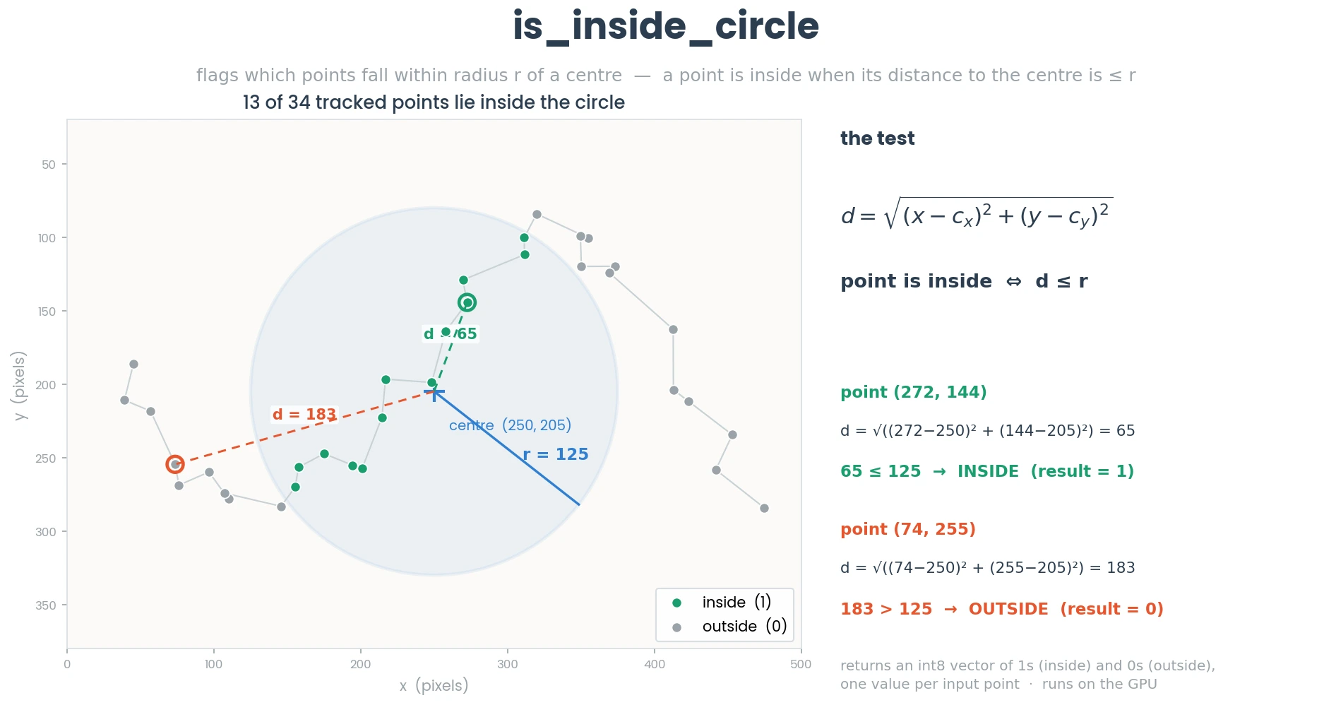

EXPECTED RUNTIMES
FRAMES (MILLIONS)	CUDA JIT GPU (S)
2	0.006
4	0.007
8	0.016
16	0.028
32	0.054
64	0.114
128	0.319
256	0.44
512	1.085
1000	2.966

Parameters

• x (np.ndarray) – 2d numeric np.ndarray size (N, 2).

• y (np.ndarray) – 2d numeric np.ndarray size (1, 2) representing the center of the circle.

• r (float) – The radius of the circle.

Returns

2d numeric boolean (N, 1) with 1s representing the point being inside the circle and 0 if the point is outside the rectangle.

Return type

1d np.ndarray vector.

simba.data_processors.cuda.geometry.is_inside_polygon(x, y)

Determines whether points in array x are inside the polygon defined by the vertices in array y.

This function uses GPU acceleration to perform the point-in-polygon test. The points in x are tested against the polygon defined by the vertices in y. The result is an array where each element indicates whether the corresponding point is inside the polygon.

EXPECTED RUNTIMES
FRAMES (MILLIONS)	CUDA JIT GPU (S)	NUMBA CPU TIME (S)
2	0.002	0.038
4	0.004	0.082
8	0.006	0.170
16	0.009	0.295
32	0.021	0.823
64	0.041	1.395
128	0.101	2.688
256	0.369	4.640
512	0.614	10.940
1000	1.293	19.947

See also

For jitted CPU function see framewise_inside_polygon_roi()

Parameters

• x (np.ndarray) – An array of shape (N, 2) where each row represents a point in 2D space. The points are checked against the polygon.

• y (np.ndarray) – An array of shape (M, 2) where each row represents a vertex of the polygon in 2D space.

Returns

An array of shape (N,) where each element is 1 if the corresponding point in x is inside the polygon defined by y, and 0 otherwise.

Return type

np.ndarray

Example

>>> x = np.random.randint(0, 200, (i, 2)).astype(np.int8)
>>> y = np.random.randint(0, 200, (4, 2)).astype(np.int8)
>>> results = is_inside_polygon(x=x, y=y)
>>> print(results)
>>> [1 0 1 0 1 1 0 0 1 0]

simba.data_processors.cuda.geometry.is_inside_rectangle(x, y)

Determines whether points in array x are inside the rectangle defined by the top left and bottom right vertices in array y. 😍

EXPECTED RUNTIMES
FRAMES (MILLIONS)	CUDA JIT GPU (S)	NUMBA CPU TIME (S)
2	0.005	0.022
4	0.009	0.031
8	0.016	0.097
16	0.028	0.199
32	0.054	0.399
64	0.111	0.769
128	0.33	1.300
256	0.666	2.531
512	1.161	7.273
1000	3.828	13.342

See also

For numba CPU function see framewise_inside_rectangle_roi()

Parameters

• x (np.ndarray) – 2d numeric np.ndarray size (N, 2).

• y (np.ndarray) – 2d numeric np.ndarray size (2, 2) (top left[x, y], bottom right[x, y])

Returns

2d numeric boolean (N, 1) with 1s representing the point being inside the rectangle and 0 if the point is outside the rectangle.

Return type

np.ndarray

simba.data_processors.cuda.geometry.poly_area(data, pixels_per_mm=1.0, batch_size=5000000)

Compute the area of a polygon using GPU acceleration.

This function calculates the area of polygons defined by sets of points in a 3D array. Each 2D slice along the first dimension represents a polygon, with each row corresponding to a point in the polygon and each column representing the x and y coordinates.

The computation is done in batches to handle large datasets efficiently.

See also

jitted_hull().

Parameters

• data – A 3D numpy array of shape (N, M, 2), where N is the number of polygons, M is the number of points per polygon, and 2 represents the x and y coordinates.

• pixels_per_mm – Optional scaling factor to convert the area from pixels squared to square millimeters. Default is 1.0.

• batch_size – Optional batch size for processing the data in chunks to fit in memory. Default is 0.5e+7.

Returns

A 1D numpy array of shape (N,) containing the computed area of each polygon in square millimeters.

Return type

np.ndarray

Image (GPU)

simba.data_processors.cuda.image.bg_subtraction_cuda(video_path, avg_frm, save_path=None, bg_clr=(0, 0, 0), fg_clr=None, batch_size=500, threshold=50)

Remove background from videos using GPU acceleration.

Note

To create an avg_frm, use simba.video_processors.video_processing.create_average_frm(), simba.data_processors.cuda.image.create_average_frm_cupy(), or create_average_frm_cuda()

See also

For CPU-based alternative, see simba.video_processors.video_processing.video_bg_subtraction() or video_bg_subtraction_mp() For GPU-based alternative, see bg_subtraction_cupy(). Needs work, CPU/multicore appears faster.

See also

To create average frame on the CPU, see simba.video_processors.video_processing.create_average_frm(). CPU/multicore appears faster.

EXPECTED RUNTIMES
FRAMES	GPU TIME (S)	GPU TIME (STEV)
450	2.76	0.18
900	5.45	0.208
1800	10.36	0.183
3600	20.527	0.886
7200	42.79	0.327
14400	82.95	3.69
28800	160.38	5.186
NVIDIA GeForce RTX 4070
video, RGB 620x530:
3 ITERATIONS

Parameters

• video_path (Union[str, os.PathLike]) – The path to the video to remove the background from.

• avg_frm (np.ndarray) – Average frame of the video. Can be created with e.g., simba.video_processors.video_processing.create_average_frm().

• save_path (Optional[Union[str, os.PathLike]]) – Optional location to store the background removed video. If None, then saved in the same directory as the input video with the _bg_removed suffix.

• bg_clr (Optional[Tuple[int, int, int]]) – Tuple representing the background color of the video.

• fg_clr (Optional[Tuple[int, int, int]]) – Tuple representing the foreground color of the video (e.g., the animal). If None, then the original pixel colors will be used. Default: 50.

• batch_size (Optional[int]) – Number of frames to process concurrently. Use higher values of RAM memory allows. Default: 500.

• threshold (Optional[int]) – Value between 0-255 representing the difference threshold between the average frame subtracted from each frame. Higher values and more pixels will be considered background. Default: 50.

Example

>>> video_path = "/mnt/c/troubleshooting/mitra/project_folder/videos/clipped/592_MA147_Gq_CNO_0515.mp4"
>>> avg_frm = create_average_frm(video_path=video_path)
>>> bg_subtraction_cuda(video_path=video_path, avg_frm=avg_frm, fg_clr=(255, 255, 255))

simba.data_processors.cuda.image.bg_subtraction_cupy(video_path, avg_frm, save_path=None, bg_clr=(0, 0, 0), fg_clr=None, batch_size=500, threshold=50, verbose=True, async_frame_read=True)

Remove background from videos using GPU acceleration through CuPY.

See also

For CPU-based alternative, see simba.video_processors.video_processing.video_bg_subtraction() or video_bg_subtraction_mp() For GPU-based alternative, see bg_subtraction_cuda(). Needs work, CPU/multicore appears faster.

Parameters

• video_path (Union[str, os.PathLike]) – The path to the video to remove the background from.

• avg_frm (np.ndarray) – Average frame of the video. Can be created with e.g., simba.video_processors.video_processing.create_average_frm().

• save_path (Optional[Union[str, os.PathLike]]) – Optional location to store the background removed video. If None, then saved in the same directory as the input video with the _bg_removed suffix.

• bg_clr (Optional[Tuple[int, int, int]]) – Tuple representing the background color of the video.

• fg_clr (Optional[Tuple[int, int, int]]) – Tuple representing the foreground color of the video (e.g., the animal). If None, then the original pixel colors will be used. Default: 50.

• batch_size (Optional[int]) – Number of frames to process concurrently. Use higher values of RAM memory allows. Default: 500.

• threshold (Optional[int]) – Value between 0-255 representing the difference threshold between the average frame subtracted from each frame. Higher values and more pixels will be considered background. Default: 50.

Example

>>> avg_frm = create_average_frm(video_path="/mnt/c/troubleshooting/mitra/project_folder/videos/temp/temp_ex_bg_subtraction/original/844_MA131_gq_CNO_0624.mp4")
>>> video_path = "/mnt/c/troubleshooting/mitra/project_folder/videos/temp/temp_ex_bg_subtraction/844_MA131_gq_CNO_0624_7.mp4"
>>> bg_subtraction_cupy(video_path=video_path, avg_frm=avg_frm, batch_size=500)

simba.data_processors.cuda.image.create_average_frm_cuda(video_path, start_frm=None, end_frm=None, start_time=None, end_time=None, save_path=None, batch_size=6000, verbose=False, async_frame_read=False)

Computes the average frame using GPU acceleration from a specified range of frames or time interval in a video file. This average frame typically used for background substraction.

The function reads frames from the video, calculates their average, and optionally saves the result to a specified file. If save_path is provided, the average frame is saved as an image file; otherwise, the average frame is returned as a NumPy array.

See also

For CuPy function see create_average_frm_cupy(). For CPU function see create_average_frm().

Parameters

• video_path (Union[str, os.PathLike]) – The path to the video file from which to extract frames.

• start_frm (Optional[int]) – The starting frame number (inclusive). Either start_frm/end_frm or start_time/end_time must be provided, but not both.

• end_frm (Optional[int]) – The ending frame number (exclusive).

• start_time (Optional[str]) – The start time in the format ‘HH:MM:SS’ from which to begin extracting frames.

• end_time (Optional[str]) – The end time in the format ‘HH:MM:SS’ up to which frames should be extracted.

• save_path (Optional[Union[str, os.PathLike]]) – The path where the average frame image will be saved. If None, the average frame is returned as a NumPy array.

• batch_size (Optional[int]) – The number of frames to process in each batch. Default is 3000. Increase if your RAM allows it.

• verbose (Optional[bool]) – If True, prints progress and informational messages during execution.

Returns

Returns None if the result is saved to save_path. Otherwise, returns the average frame as a NumPy array.

Example

>>> create_average_frm_cuda(video_path=r"C:/troubleshooting/RAT_NOR/project_folder/videos/2022-06-20_NOB_DOT_4_downsampled.mp4", verbose=True, start_frm=0, end_frm=9000)

simba.data_processors.cuda.image.create_average_frm_cupy(video_path, start_frm=None, end_frm=None, start_time=None, end_time=None, save_path=None, batch_size=3000, verbose=False, async_frame_read=False)

Computes the average frame using GPU acceleration from a specified range of frames or time interval in a video file. This average frame is typically used for background subtraction.

The function reads frames from the video, calculates their average, and optionally saves the result to a specified file. If save_path is provided, the average frame is saved as an image file; otherwise, the average frame is returned as a NumPy array.

See also

For CPU function see create_average_frm(). For CUDA function see create_average_frm_cuda()

EXPECTED RUNTIMES
OBSERVATIONS (THOUSANDS)	TIME (S)	STDEV (S)
1	2.323333333	0.032145503
2	3.486666667	0.205993527
3	4.71	0.02
4	6.03	0.346987031
5	7.566666667	0.159478316
6	8.943333333	0.210792157
7	10.26666667	0.494098506
NVIDIA GeForce RTX 4070
REPEATS = 3
BATCH SIZE: 500.
RESOLUTION: 600 x 400
ASYNC FRAME READ: TRUE

Parameters

• video_path (Union[str, os.PathLike]) – The path to the video file from which to extract frames.

• start_frm (Optional[int]) – The starting frame number (inclusive). Either start_frm/end_frm or start_time/end_time must be provided, but not both. If both start_frm and end_frm are None, processes all frames in the video.

• end_frm (Optional[int]) – The ending frame number (exclusive). Either start_frm/end_frm or start_time/end_time must be provided, but not both.

• start_time (Optional[str]) – The start time in the format ‘HH:MM:SS’ from which to begin extracting frames. Either start_frm/end_frm or start_time/end_time must be provided, but not both.

• end_time (Optional[str]) – The end time in the format ‘HH:MM:SS’ up to which frames should be extracted. Either start_frm/end_frm or start_time/end_time must be provided, but not both.

• save_path (Optional[Union[str, os.PathLike]]) – The path where the average frame image will be saved. If None, the average frame is returned as a NumPy array.

• batch_size (Optional[int]) – The number of frames to process in each batch. Default is 3000. Increase if your RAM allows it.

• verbose (Optional[bool]) – If True, prints progress and informational messages during execution. Default: False.

• async_frame_read (bool) – If True, uses asynchronous frame reading for improved performance. Default: False.

Returns

Returns None if the result is saved to save_path. Otherwise, returns the average frame as a NumPy array.

Example

>>> create_average_frm_cupy(video_path=r"C:/troubleshooting/RAT_NOR/project_folder/videos/2022-06-20_NOB_DOT_4_downsampled.mp4", verbose=True, start_frm=0, end_frm=9000)
>>> create_average_frm_cupy(video_path=r"C:/videos/my_video.mp4", start_time="00:00:00", end_time="00:01:00", async_frame_read=True, save_path=r"C:/output/avg_frame.png")

simba.data_processors.cuda.image.img_stack_brightness(x, method='digital', ignore_black=True, verbose=False, batch_size=2500)

Calculate the average brightness of a stack of images using a specified method.

Useful for analyzing light cues or brightness changes over time. For example, compute brightness in images containing a light cue ROI, then perform clustering (e.g., k-means) on brightness values to identify frames when the light cue is on vs off.

EXPECTED RUNTIMES
FRAME COUNT (K)	TIME (SECONDS)	STDEV (SECONDS)
1	0.76485	1.239735707
5	3.9256	10.04421855
7	9.445	11.46390422
RESOLUTON: 1200x600
3 RUNS
RTX 4090

• Photometric Method: The brightness is calculated using the formula:

\[\text{brightness} = 0.2126 \cdot R + 0.7152 \cdot G + 0.0722 \cdot B\]

• Digital Method: The brightness is calculated using the formula:

\[\text{brightness} = 0.299 \cdot R + 0.587 \cdot G + 0.114 \cdot B\]

See also

For CPU function see brightness_intensity().

Parameters

• x (np.ndarray) – A 4D array of images with dimensions (N, H, W, C), where N is the number of images, H and W are the height and width, and C is the number of channels (RGB).

• method (Optional[Literal['photometric', 'digital']]) – The method to use for calculating brightness. It can be ‘photometric’ for the standard luminance calculation or ‘digital’ for an alternative set of coefficients. Default is ‘digital’.

• ignore_black (Optional[bool]) – If True, black pixels (i.e., pixels with brightness value 0) will be ignored in the calculation of the average brightness. Default is True.

Return np.ndarray

A 1D array of average brightness values for each image in the stack. If ignore_black is True, black pixels are ignored in the averaging process.

Example

>>> imgs = read_img_batch_from_video_gpu(video_path=r"/mnt/c/troubleshooting/RAT_NOR/project_folder/videos/2022-06-20_NOB_DOT_4_downsampled.mp4", start_frm=0, end_frm=5000)
>>> imgs = np.stack(list(imgs.values()), axis=0)
>>> x = img_stack_brightness(x=imgs)

simba.data_processors.cuda.image.img_stack_to_bw(imgs, lower_thresh=100, upper_thresh=100, invert=True, batch_size=1000)

Converts a stack of RGB images to binary (black and white) images based on given threshold values using GPU acceleration.

This function processes a 4D stack of images, converting each RGB image to a binary image using specified lower and upper threshold values. The conversion can be inverted if desired, and the processing is done in batches for efficiency.

EXPECTED RUNTIMES
FRAMES (K)	TIME (S)
1	0.280
2	0.260
4	0.600
8	1.100

See also

simba.mixins.image_mixin.ImageMixin.img_to_bw() simba.mixins.image_mixin.ImageMixin.img_stack_to_bw()

Parameters

• imgs (np.ndarray) – A 4D NumPy array representing a stack of RGB images, with shape (N, H, W, C).

• lower_thresh (Optional[int]) – The lower threshold value. Pixel values below this threshold are set to 0 (or 1 if invert is True). Default is 100.

• upper_thresh (Optional[int]) – The upper threshold value. Pixel values above this threshold are set to 1 (or 0 if invert is True). Default is 100.

• invert (Optional[bool]) – If True, the binary conversion is inverted, meaning that values below lower_thresh become 1, and values above upper_thresh become 0. Default is True.

• batch_size (Optional[int]) – The number of images to process in a single batch. This helps manage memory usage for large stacks of images. Default is 1000.

Returns

A 3D NumPy array of shape (N, H, W), where each image has been converted to a binary format with pixel values of either 0 or 1.

Return type

np.ndarray

simba.data_processors.cuda.image.img_stack_to_grayscale_cuda(x)

Convert image stack to grayscale using CUDA.

See also

For CPU function single images img_to_greyscale() and img_stack_to_greyscale() for stack. For CuPy, see img_stack_to_grayscale_cupy().

EXPECTED RUNTIMES
FRAMES (k)	GPU (s)	STDEV (s)
1	0.16022	0.125786
2	0.14428	0.003726
3	0.19769	0.005645
4	0.2571	0.006002
5	0.33574	0.017868
6	0.39921	0.026858
7	0.45734	0.0333
8	0.53216	0.015075
9	0.50257	0.023186
10	0.54235	0.090055
11	0.69896	0.00999
12	0.57932	0.0010399
13	0.63791	0.017
14	0.99677	0.1073426
15	1.56103	0.5308574
16	1.08143	0.082
17	1.39189	0.3308389
18	1.23648	0.1386822
19	1.39554	0.161
20	1.962	0.576
NVIDIA GeForce RTX 4070
REPEATS= 3

Parameters

x (np.ndarray) – 4d array of color images in numpy format.

Return np.ndarray

3D array of greyscaled images.

Example

>>> imgs = read_img_batch_from_video_gpu(video_path=r"/mnt/c/troubleshooting/mitra/project_folder/videos/temp_2/592_MA147_Gq_Saline_0516_downsampled.mp4", verbose=False, start_frm=0, end_frm=i)
>>> imgs = np.stack(list(imgs.values()), axis=0).astype(np.uint8)
>>> grey_images = img_stack_to_grayscale_cuda(x=imgs)

simba.data_processors.cuda.image.img_stack_to_grayscale_cupy(imgs, batch_size=250)

Converts a stack of color images to grayscale using GPU acceleration with CuPy.

See also

For CPU function single images img_to_greyscale() and img_stack_to_greyscale() for stack. For CUDA JIT, see img_stack_to_grayscale_cuda().

EXPECTED RUNTIMES
FRAMES (THOUSANDS)	GPU (s)
0.5	0.3419
1	0.52333
1.5	0.81614
2	1.0632
2.5	1.32399
3	1.61488
3.5	1.87857
4	2.30137
4.5	2.54736
5	2.90824
5.5	3.09271

Parameters

• imgs (np.ndarray) – A 4D NumPy or CuPy array representing a stack of images with shape (num_images, height, width, channels). The images are expected to have 3 channels (RGB).

• batch_size (Optional[int]) – The number of images to process in each batch. Defaults to 250. Adjust this parameter to fit your GPU’s memory capacity.

Return np.ndarray

m A 3D NumPy or CuPy array of shape (num_images, height, width) containing the grayscale images. If the input array is not 4D, the function returns the input as is.

Example

>>> imgs = read_img_batch_from_video_gpu(video_path=r"/mnt/c/troubleshooting/RAT_NOR/project_folder/videos/2022-06-20_NOB_IOT_1_cropped.mp4", verbose=False, start_frm=0, end_frm=i)
>>> imgs = np.stack(list(imgs.values()), axis=0).astype(np.uint8)
>>> gray_imgs = img_stack_to_grayscale_cupy(imgs=imgs)

simba.data_processors.cuda.image.pose_plotter(data, video_path, save_path, circle_size=None, colors='Set1', batch_size=750, verbose=True)

Creates a video overlaying pose-estimation data on frames from a given video using GPU acceleration.

See also

For CPU based methods, see PathPlotterSingleCore() and PathPlotterMulticore().

EXPECTED RUNTIMES
FRAMES (K)	TIME (S)
4	17
6	27
10	36
18	63
26	93
NVIDIA GeForce RTX 4070
7 body-parts
FRAME SIZE (WxH): 726x538
BATCH SIZE: 1000 images

Parameters

• data (Union[str, os.PathLike, np.ndarray]) – Path to a CSV file with pose-estimation data or a 3d numpy array (n_images, n_bodyparts, 2) with pose-estimated locations.

• video_path (Union[str, os.PathLike]) – Path to a video file where the data has been pose-estimated.

• save_path (Union[str, os.PathLike]) – Location where to store the output visualization.

• circle_size (Optional[int]) – The size of the circles representing the location of the pose-estimated locations. If None, the optimal size will be inferred as a 100th of the max(resultion_w, h).

• batch_size (int) – The number of frames to process concurrently on the GPU. Default: 750. Increase of host and device RAM allows it to improve runtime. Decrease if you hit memory errors.

Example

>>> DATA_PATH = "/mnt/c/troubleshooting/mitra/project_folder/csv/outlier_corrected_movement_location/501_MA142_Gi_CNO_0521.csv"
>>> VIDEO_PATH = "/mnt/c/troubleshooting/mitra/project_folder/videos/501_MA142_Gi_CNO_0521.mp4"
>>> SAVE_PATH = "/mnt/c/troubleshooting/mitra/project_folder/frames/output/pose_ex/test.mp4"
>>> pose_plotter(data=DATA_PATH, video_path=VIDEO_PATH, save_path=SAVE_PATH, circle_size=10, batch_size=1000)

simba.data_processors.cuda.image.rotate_img_stack_cupy(imgs, rotation_degrees=180, batch_size=500, verbose=True)

Rotates a stack of images by a specified number of degrees using GPU acceleration with CuPy.

Accepts a 3D (single-channel images) or 4D (multichannel images) NumPy array, rotates each image in the stack by the specified degree around the center, and returns the result as a NumPy array.

Parameters

• imgs (np.ndarray) – The input stack of images to be rotated. Expected to be a NumPy array with 3 or 4 dimensions. 3D shape: (num_images, height, width) - 4D shape: (num_images, height, width, channels)

• rotation_degrees (Optional[float]) – The angle by which the images should be rotated, in degrees. Must be between 1 and 359 degrees. Defaults to 180 degrees.

• batch_size (Optional[int]) – Number of images to process on GPU in each batch. Decrease if data can’t fit on GPU RAM.

Returns

A NumPy array containing the rotated images with the same shape as the input.

Return type

np.ndarray

Example

>>> video_path = r"/mnt/c/troubleshooting/mitra/project_folder/videos/F0_gq_Saline_0626_clipped.mp4"
>>> imgs = read_img_batch_from_video_gpu(video_path=video_path)
>>> imgs = np.stack(np.array(list(imgs.values())), axis=0)
>>> imgs = rotate_img_stack_cupy(imgs=imgs, rotation=50)

simba.data_processors.cuda.image.rotate_video_cupy(video_path, save_path=None, rotation_degrees=180, batch_size=None, verbose=True)

Rotates a video by a specified angle using GPU acceleration and CuPy for image processing.

Parameters

• video_path (Union[str, os.PathLike]) – Path to the input video file.

• save_path (Optional[Union[str, os.PathLike]]) – Path to save the rotated video. If None, saves the video in the same directory as the input with ‘_rotated_<rotation_degrees>’ appended to the filename.

• rotation_degrees (nptional[float]) – Degrees to rotate the video. Must be between 1 and 359 degrees. Default is 180.

• batch_size (Optional[int]) – The number of frames to process in each batch. Deafults to None meaning all images will be processed in a single batch.

Returns

None.

Example

>>> video_path = r"/mnt/c/troubleshooting/mitra/project_folder/videos/F0_gq_Saline_0626_clipped.mp4"
>>> rotate_video_cupy(video_path=video_path, rotation_degrees=45)

simba.data_processors.cuda.image.segment_img_stack_horizontal(imgs, pct, upper=False, lower=False)

Segment a stack of images horizontally based on a given percentage using GPU acceleration. For example, return the top half, bottom half, or center half of each image in the stack.

Note

If both top and bottom are true, the center portion is returned.

See also

simba.mixins.image_mixin.ImageMixin.segment_img_stack_horizontal()

Parameters

• imgs (np.ndarray) – A 3D or 4D NumPy array representing a stack of images. The array should have shape (N, H, W) for grayscale images or (N, H, W, C) for color images.

• pct (float) – The percentage of the image width to be used for segmentation. This value should be between a small positive value (e.g., 10e-6) and 0.99.

• upper (bool) – If True, the top part of the image stack will be segmented.

• lower (bool) – If True, the bottom part of the image stack will be segmented.

Returns

A NumPy array containing the segmented images, with the same number of dimensions as the input.

Return type

np.ndarray

simba.data_processors.cuda.image.segment_img_stack_vertical(imgs, pct, left, right)

Segment a stack of images vertically based on a given percentage using GPU acceleration. For example, return the left half, right half, or senter half of each image in the stack.

Note

If both left and right are true, the center portion is returned.

See also

simba.mixins.image_mixin.ImageMixin.segment_img_vertical()

Parameters

• imgs (np.ndarray) – A 3D or 4D NumPy array representing a stack of images. The array should have shape (N, H, W) for grayscale images or (N, H, W, C) for color images.

• pct (float) – The percentage of the image width to be used for segmentation. This value should be between a small positive value (e.g., 10e-6) and 0.99.

• left (bool) – If True, the left side of the image stack will be segmented.

• right (bool) – If True, the right side of the image stack will be segmented.

Returns

A NumPy array containing the segmented images, with the same number of dimensions as the input.

Return type

np.ndarray

simba.data_processors.cuda.image.slice_imgs(video_path, shapes, batch_size=1000, verbose=True, save_dir=None)

Slice frames from a video based on given polygon or circle coordinates, and return or save masked/cropped frame regions using GPU acceleration.

This function supports two types of shapes:

• Polygon: array of shape (N, M, 2), where N = number of frames, M = number of polygon vertices.

• Circle: array of shape (N, 3), where each row represents [center_x, center_y, radius].

Parameters

• video_path (Union[str, os.PathLike]) – Path to the input video file.

• shapes (np.ndarray) – Array of polygon coordinates or circle parameters for each frame. - Polygon: shape = (n_frames, n_vertices, 2) - Circle: shape = (n_frames, 3)

• batch_size (int) – Number of frames to process per batch during GPU processing. Default 1000.

• verbose (bool) – Whether to print progress and status messages. Default True.

• save_dir (Optional[Union[str, os.PathLike]]) – If provided, the masked/cropped video will be saved in this directory. Otherwise, the cropped image stack will be returned.

EXPECTED RUNTIMES
FRAMES N	TIME (S)
500	2.92
1000	2.134
2000	3.881
4000	7.358
8000	15.066
16000	35.156
32000	57.9812
IMG SIZE: 714 x 528

Note

For CPU multicore implementation, see simba.mixins.image_mixin.ImageMixin.slice_shapes_in_imgs(). For single core process, see simba.mixins.image_mixin.ImageMixin.slice_shapes_in_img()

Example I

Example 1: Mask video using circular regions derived from body part center positions >>> video_path = “/mnt/c/troubleshooting/RAT_NOR/project_folder/videos/03152021_NOB_IOT_8.mp4” >>> data_path = “/mnt/c/troubleshooting/RAT_NOR/project_folder/csv/outlier_corrected_movement_location/03152021_NOB_IOT_8.csv” >>> save_dir = ‘/mnt/d/netholabs/yolo_videos/input/mp4_20250606083508’ >>> nose_arr = read_df(file_path=data_path, file_type=’csv’, usecols=[‘Nose_x’, ‘Nose_y’]).values.reshape(-1, 2).astype(np.int32) >>> polygons = GeometryMixin().multiframe_bodyparts_to_circle(data=nose_arr, parallel_offset=60) >>> polygon_lst = [] >>> center = GeometryMixin.get_center(polygons) >>> polygons = np.hstack([center, np.full(shape=(len(center), 1), fill_value=60)]) >>> slice_imgs(video_path=video_path, shapes=polygons, batch_size=500, save_dir=save_dir)

Example II

Example 2: Mask video using minimum rotated rectangles from polygon hulls

>>> video_path = "/mnt/c/troubleshooting/RAT_NOR/project_folder/videos/03152021_NOB_IOT_8.mp4"
>>> data_path = "/mnt/c/troubleshooting/RAT_NOR/project_folder/csv/outlier_corrected_movement_location/03152021_NOB_IOT_8.csv"
>>> save_dir = '/mnt/d/netholabs/yolo_videos/input/mp4_20250606083508'
>>> nose_arr = read_df(file_path=data_path, file_type='csv', usecols=['Nose_x', 'Nose_y', 'Tail_base_x', 'Tail_base_y', 'Lat_left_x', 'Lat_left_y', 'Lat_right_x', 'Lat_right_y']).values.reshape(-1, 4, 2).astype(np.int32) ## READ THE BODY-PART THAT DEFINES THE HULL AND CONVERT TO ARRAY
>>> polygons = GeometryMixin().multiframe_bodyparts_to_polygon(data=nose_arr, parallel_offset=60)
>>> polygons = GeometryMixin().multiframe_minimum_rotated_rectangle(shapes=polygons)
>>> polygon_lst = []
>>> for i in polygons:
>>> polygon_lst.append(np.array(i.exterior.coords).astype(np.int32))
>>> polygons = np.stack(polygon_lst, axis=0)
>>> sliced_imgs = slice_imgs(video_path=video_path, shapes=polygons, batch_size=500, save_dir=save_dir)

simba.data_processors.cuda.image.sliding_psnr(data, stride_s, sample_rate)

Computes the Peak Signal-to-Noise Ratio (PSNR) between pairs of images in a stack using a sliding window approach.

This function calculates PSNR for each image in a stack compared to another image in the stack that is separated by a specified stride. The sliding window approach allows for the comparison of image quality over a sequence of images.

Note

• PSNR values are measured in decibels (dB).

• Higher PSNR values indicate better quality with minimal differences from the reference image.

• Lower PSNR values indicate higher distortion or noise.

\[\text{PSNR} = 20 \log_{10} \left( \frac{\text{MAX}}{\sqrt{\text{MSE}}} \right)\]

where: - \(\text{MAX}\) is the maximum possible pixel value (255 for 8-bit images) - \(\text{MSE}\) is the Mean Squared Error between the two images

Parameters

• data – A 4D NumPy array of shape (N, H, W, C) representing a stack of images, where N is the number of images, H is the height, W is the width, and C is the number of color channels.

• stride_s – The base stride length in terms of the number of images between the images being compared. Determines the separation between images for comparison in the stack.

• sample_rate – The sample rate to scale the stride length. This allows for adjusting the stride dynamically based on the sample rate.

Returns

A 1D NumPy array of PSNR values, where each element represents the PSNR between the image at index r and the image at index l = r - stride, for all valid indices r.

Return type

np.ndarray

Example

>>> data = ImageMixin().read_img_batch_from_video(video_path =r"/mnt/c/troubleshooting/mitra/project_folder/videos/clipped/501_MA142_Gi_CNO_0514_clipped.mp4", start_frm=0, end_frm=299)
>>> data = np.stack(list(data.values()), axis=0).astype(np.uint8)
>>> data = ImageMixin.img_stack_to_greyscale(imgs=data)
>>> p = sliding_psnr(data=data, stride_s=1, sample_rate=1)

simba.data_processors.cuda.image.stack_sliding_mse(x, stride=1, batch_size=1000)

Computes the Mean Squared Error (MSE) between each image in a stack and a reference image, where the reference image is determined by a sliding window approach with a specified stride. The function is optimized for large image stacks by processing them in batches.

See also

For CPU function see img_stack_mse() and img_sliding_mse().

\[\text{MSE} = \frac{1}{n} \sum_{i=1}^{n} (y_i - \hat{y}_i)^2\]

Parameters

• x (np.ndarray) – Input array of images, where the first dimension corresponds to the stack of images. The array should be either 3D (height, width, channels) or 4D (batch, height, width, channels).

• stride (Optional[int]) – The stride or step size for the sliding window that determines the reference image. Defaults to 1, meaning the previous image in the stack is used as the reference.

• batch_size (Optional[int]) – The number of images to process in a single batch. Larger batch sizes may improve performance but require more GPU memory. Defaults to 1000.

Returns

A 1D NumPy array containing the MSE for each image in the stack compared to its corresponding reference image. The length of the array is equal to the number of images in the input stack.

Return type

np.ndarray

Statistics (GPU)

simba.data_processors.cuda.statistics.adjusted_rand_gpu(x, y)

Calculate the Adjusted Rand Index (ARI) between two clusterings.

The Adjusted Rand Index (ARI) is a measure of the similarity between two clusterings. It considers all pairs of samples and counts pairs that are assigned to the same or different clusters in both the true and predicted clusterings.

The ARI is defined as:

\[ARI = \frac{TP + TN}{TP + FP + FN + TN}\]

where:

• \(TP\) (True Positive) is the number of pairs of elements that are in the same cluster in both x and y,

• \(FP\) (False Positive) is the number of pairs of elements that are in the same cluster in y but not in x,

• \(FN\) (False Negative) is the number of pairs of elements that are in the same cluster in x but not in y,

• \(TN\) (True Negative) is the number of pairs of elements that are in different clusters in both x and y.

The ARI value ranges from -1 to 1. A value of 1 indicates perfect clustering agreement, 0 indicates random clustering, and negative values indicate disagreement between the clusterings.

Note

Modified from scikit-learn

See also

For CPU call, see simba.mixins.statistics_mixin.Statistics.adjusted_rand().

Parameters

• x (np.ndarray) – 1D array representing the labels of the first model.

• y (np.ndarray) – 1D array representing the labels of the second model.

Returns

A value of 1 indicates perfect clustering agreement, a value of 0 indicates random clustering, and negative values indicate disagreement between the clusterings.

Return type

float

Example

>>> x = np.random.randint(low=0, high=55, size=100000000)
>>> y = np.random.randint(low=0, high=55, size=100000000)
>>> adjusted_rand_gpu(x=x, y=y)

simba.data_processors.cuda.statistics.count_values_in_ranges(x, r)

Counts the number of values in each feature within specified ranges for each row in a 2D array using CUDA.

EXPECTED RUNTIMES
FRAMES (MILLION)	TIME (S)
4	0.038
8	0.201
16	0.344
32	0.306
64	0.776
128	1.611
NVIDIA GeForce RTX 4070
(n, 11)

See also

For CPU function see count_values_in_range().

Parameters

• x (np.ndarray) – 2d array with feature values.

• r (np.ndarray) – 2d array with lower and upper boundaries.

Returns

2d array of size len(x) x len(r) with the counts of values in each feature range (inclusive).

Return type

np.ndarray

Example

>>> x = np.random.randint(1, 11, (10, 10)).astype(np.int8)
>>> r = np.array([[1, 6], [6, 11]])
>>> r_x = count_values_in_ranges(x=x, r=r)

simba.data_processors.cuda.statistics.davis_bouldin(x, y)

Computes the Davis-Bouldin Index using GPU acceleration, a clustering evaluation metric that assesses the quality of clustering based on the ratio of within-cluster and between-cluster distances.

The lower the Davis-Bouldin Index, the better the clusters are separated and compact. The function calculates the average similarity between each cluster and its most similar cluster.

See also

For CPU implementation, use simba.mixins.statistics_mixin.Statistics.davis_bouldin()

EXPECTED RUNTIMES
OBSERVATIONS (MILLIONS)	TIME (S)	STDEV (S)
2	0.03166	0.023
4	0.06161	0.04883
8	0.12143	0.09597
16	0.24169	0.19592
32	0.27942	0.12019
64	0.45187	0.09255
128	0.98631	0.31372
NVIDIA GeForce RTX 4070
REPEATS = 3
centers = [[0, 0], [5, 10], [10, 0], [20, 10]]
x, y = make_blobs(n_samples=OBSERVATIONS, n_features=2, centers=centers, cluster_std=1)

Parameters

• x (np.ndarray) – A 2D array of data points where each row corresponds to aan observation and each column corresponds to a feature.

• y (np.ndarray) – A 1D array containing the cluster labels for each sample in x.

Returns

The Davis-Bouldin Index as a float, where lower values indicate better-defined clusters.

Return type

float

Example

>>> centers = [[0, 0], [5, 10], [10, 0], [20, 10]]  # Adjust distances between cluster centers
>>> x, y = make_blobs(n_samples=50000, n_features=4, centers=3, cluster_std=0.1)
>>> p = davis_bouldin(x, y)

simba.data_processors.cuda.statistics.dunn_index(x, y)

Computes the Dunn Index for clustering quality using GPU acceleration, which is a ratio of the minimum inter-cluster distance to the maximum intra-cluster distance. The higher the Dunn Index, the better the separation between clusters.

The Dunn Index is given by:

\[D = \frac{\min_{i \neq j} \{ \delta(C_i, C_j) \}}{\max_k \{ \Delta(C_k) \}}\]

where \(\delta(C_i, C_j)\) is the distance between clusters \(C_i\) and \(C_j\), and \(\Delta(C_k)\) is the diameter of cluster \(C_k\).

The higher the Dunn Index, the better the clustering, as a higher value indicates that the clusters are well-separated relative to their internal cohesion.

EXPECTED RUNTIMES
OBSERVATIONS (MILLIONS)	TIME (S)	STDEV (S)
2	0.2366	0.0114
4	0.4464	0.0016
8	0.9037	0.0032
16	1.8675	0.0019
32	3.6247	0.006497
64	7.2898	0.007388
128	14.822	0.02672
256	29.316	0.0425
512	58.23599271	0.477388716
NVIDIA GeForce RTX 4070
REPEATS = 3
centers = [[0, 0], [5, 10], [10, 0], [20, 10]]
x, y = make_blobs(n_samples=OBSERVATIONS, n_features=2, centers=centers, cluster_std=1)

Parameters

• x (np.ndarray) – The input data points, where each row corresponds to an observation, and columns are features.

• y (np.ndarray) – Cluster labels for the data points. Each label corresponds to a cluster assignment for the respective observation in x.

Returns

The Dunn Index, a floating point value that measures the quality of clustering.

Return type

float

Example

>>> centers = [[0, 0], [5, 10], [10, 0], [20, 10]]  # Adjust distances between cluster centers
>>> x, y = make_blobs(n_samples=80_000_000, n_features=10, centers=centers, cluster_std=1, random_state=10)
>>> v = dunn_index(x=x, y=y)

simba.data_processors.cuda.statistics.euclidean_distance_to_static_point(data, point, pixels_per_millimeter=1, centimeter=False, batch_size=65000000)

Computes the Euclidean distance between each point in a given 2D array data and a static point using GPU acceleration.

See also

For CPU-based distance to static point (ROI center), see simba.mixins.feature_extraction_mixin.FeatureExtractionMixin.framewise_euclidean_distance_roi() For CPU-based framewise Euclidean distance, see simba.mixins.feature_extraction_mixin.FeatureExtractionMixin.framewise_euclidean_distance() For GPU CuPy solution for distance between two sets of points, see simba.data_processors.cuda.statistics.get_euclidean_distance_cupy() For GPU numba CUDA solution for distance between two sets of points, see simba.data_processors.cuda.statistics.get_euclidean_distance_cuda()

Parameters

• data – A 2D array of shape (N, 2), where N is the number of points, and each point is represented by its (x, y) coordinates. The array can represent pixel coordinates.

• point – A tuple of two integers representing the static point (x, y) in the same space as data.

• pixels_per_millimeter – A scaling factor that indicates how many pixels correspond to one millimeter. Defaults to 1 if no scaling is necessary.

• centimeter – A flag to indicate whether the output distances should be converted from millimeters to centimeters. If True, the result is divided by 10. Defaults to False (millimeters).

• batch_size – The number of points to process in each batch to avoid memory overflow on the GPU. The default batch size is set to 65 million points (6.5e+7). Adjust this parameter based on GPU memory capacity.

Returns

A 1D array of distances between each point in data and the static point, either in millimeters or centimeters depending on the centimeter flag.

Return type

np.ndarray

simba.data_processors.cuda.statistics.get_3pt_angle(x, y, z)

Computes the angle formed by three points in 2D space for each corresponding row in the input arrays using GPU. The points x, y, and z represent the coordinates of three points in space, and the angle is calculated at point y between the line segments xy and yz.

EXPECTED RUNTIMES
FRAMES	TIME (S)
4 million	0.02
8 million	0.04
16 million	0.159
32 million	0.29
64 million	0.335
128 million	0.792
256 million	1.371

See also

For CPU function see angle3pt() and For CPU function see angle3pt_serialized().

Parameters

• x – A numpy array of shape (n, 2) representing the first point (e.g., nose) coordinates.

• y – A numpy array of shape (n, 2) representing the second point (e.g., center) coordinates, where the angle is computed.

• z – A numpy array of shape (n, 2) representing the second point (e.g., center) coordinates, where the angle is computed.

Returns

A numpy array of shape (n, 1) containing the calculated angles (in degrees) for each row.

Return type

np.ndarray

Example

>>> video_path = r"/mnt/c/troubleshooting/mitra/project_folder/videos/501_MA142_Gi_CNO_0514.mp4"
>>> data_path = r"/mnt/c/troubleshooting/mitra/project_folder/csv/outlier_corrected_movement_location/501_MA142_Gi_CNO_0514 - test.csv"
>>> df = read_df(file_path=data_path, file_type='csv')
>>> y = df[['Center_x', 'Center_y']].values
>>> x = df[['Nose_x', 'Nose_y']].values
>>> z = df[['Tail_base_x', 'Tail_base_y']].values
>>> angle_x = get_3pt_angle(x=x, y=y, z=z)

simba.data_processors.cuda.statistics.get_euclidean_distance_cuda(x, y)

Computes the Euclidean distance between two sets of points using CUDA for GPU acceleration.

EXPECTED RUNTIMES
OBSERVATION	TIME (S)
110k	0.007
181k	0.021
327k	0.032
620k	0.02
1.2m	0.082
2.4m	0.046
4.7m	0.106
9.3m	0.209
18.6m	0.238
37.2m	0.926
74.5m	1.136
149m	2.046

See also

For CPU function see framewise_euclidean_distance(). For CuPY function see get_euclidean_distance_cupy().

Parameters

• x (np.ndarray) – A 2D array of shape (n, m) representing n points in m-dimensional space. Each row corresponds to a point.

• y (np.ndarray) – A 2D array of shape (n, m) representing n points in m-dimensional space. Each row corresponds to a point.

Return np.ndarray

A 1D array of shape (n,) where each element represents the Euclidean distance between the corresponding points in x and y.

Example

>>> video_path = r"/mnt/c/troubleshooting/mitra/project_folder/videos/501_MA142_Gi_CNO_0514.mp4"
>>> data_path = r"/mnt/c/troubleshooting/mitra/project_folder/csv/outlier_corrected_movement_location/501_MA142_Gi_CNO_0514 - test.csv"
>>> df = read_df(file_path=data_path, file_type='csv')[['Center_x', 'Center_y']]
>>> shifted_df = FeatureExtractionMixin.create_shifted_df(df=df, periods=1)
>>> x = shifted_df[['Center_x', 'Center_y']].values
>>> y = shifted_df[['Center_x_shifted', 'Center_y_shifted']].values
>>> get_euclidean_distance_cuda(x=x, y=y)

simba.data_processors.cuda.statistics.get_euclidean_distance_cupy(x, y, batch_size=35000000007)

Computes the Euclidean distance between corresponding pairs of points in two 2D arrays using CuPy for GPU acceleration. The computation is performed in batches to handle large datasets efficiently.

See also

For CPU function see framewise_euclidean_distance(). For CUDA JIT function see get_euclidean_distance_cuda().

Parameters

• x (np.ndarray) – A 2D NumPy array with shape (n, 2), where each row represents a point in a 2D space.

• y (np.ndarray) – A 2D NumPy array with shape (n, 2), where each row represents a point in a 2D space. The shape of y must match the shape of x.

• batch_size (Optional[int]) – The number of points to process in a single batch. This parameter controls memory usage and can be adjusted based on available GPU memory. The default value is large (3.5e10 + 7) to maximize GPU utilization, but it can be lowered if memory issues arise.

Returns

A 1D NumPy array of shape (n,) containing the Euclidean distances between corresponding points in x and y.

Return type

np.ndarray

Example

>>> x = np.array([[1, 2], [3, 4], [5, 6]])
>>> y = np.array([[7, 8], [9, 10], [11, 12]])
>>> distances = get_euclidean_distance_cupy(x, y)

simba.data_processors.cuda.statistics.hamming_distance_gpu(x, y, w=None)

Computes the weighted Hamming distance between two arrays using GPU acceleration.

EXPECTED RUNTIMES
OBSERVATIONS (COUNT)	GPU TIME (S) (NUMBA CUDA)	CPU TIME (S) (NUMBA NJIT)
10k	0.01209025	0.00057592
100k	0.00364709	0.00553586
1m	0.0223	0.0551
10m	0.152	0.771
100m	0.4393	5.858
250m	1.3283	14.8490987
500m	2.2082	29.562
1tn	4.821	59.8388138
NVIDIA GeForce RTX 4070, 32 CORES

See also

For jitted CPU method, see simba.mixins.statistics_mixin.Statistics.hamming_distance().

Parameters

• x (ndarray) – A 1D or 2D NumPy array representing the reference data. If 2D, shape should be (n_samples, n_features). Supported dtypes are numeric.

• y (ndarray) – Array of the same shape as x representing the data to compare.

• w (ndarray) – A 1D array of shape (n_samples,) representing sample weights. If None, uniform weights are used.

Returns

The weighted average Hamming distance between corresponding rows of x and y.

Return type

float

Example

>>> x, y = np.random.randint(0, 2, (10, 1)).astype(np.int8), np.random.randint(0, 2, (10, 1)).astype(np.int8)
>>> gpu_hamming = hamming_distance_gpu(x=x, y=y)

simba.data_processors.cuda.statistics.i_index(x, y, verbose=False)

Calculate the I-Index for evaluating clustering quality.

The I-Index is a metric that measures the compactness and separation of clusters. A higher I-Index indicates better clustering with compact and well-separated clusters.

EXPECTED RUNTIMES
OBSERVATIONS (MILLIONS)	TIME (S)	STD TIME(S)
5	1.501366667	0.096872717
10	3.0527	0.117796944
20	5.9634	0.282048418
40	11.44683333	0.087952051
80	22.74773333	0.110135477
160	49.425	0.420928735
NVIDIA GeForce RTX 4070
7 body-parts
100 clusters / 3 features

The I-Index is calculated as:

\[I = \frac{SST}{k \times SWC}\]

where:

• \(SST = \sum_{i=1}^{n} \|x_i - \mu\|^2\) is the total sum of squares (sum of squared distances from all points to the global centroid)

• \(k\) is the number of clusters

• \(SWC = \sum_{c=1}^{k} \sum_{i \in c} \|x_i - \mu_c\|^2\) is the within-cluster sum of squares (sum of squared distances from points to their cluster centroids)

See also

To compute Xie-Beni on the CPU, use i_index()

Parameters

• x (np.ndarray) – The dataset as a 2D NumPy array of shape (n_samples, n_features).

• y (np.ndarray) – Cluster labels for each data point as a 1D NumPy array of shape (n_samples,).

Returns

The I-index score for the dataset.

Return type

float

References

1

Zhao, Q., Xu, M., & Fränti, P. (2009). Sum-of-squares based cluster validity index and significance analysis. In Adaptive and Natural Computing Algorithms (ICANNGA 2009), Lecture Notes in Computer Science, vol. 5495. Springer.

Example

>>> X, y = make_blobs(n_samples=5000, centers=20, n_features=3, random_state=0, cluster_std=0.1)
>>> i_index(x=X, y=y)

simba.data_processors.cuda.statistics.kmeans_cuml(data, k=2, max_iter=300, output_type=None, sample_n=None)

CRAP, SLOWER THAN SCIKIT

simba.data_processors.cuda.statistics.kullback_leibler_divergence_gpu(x, y, fill_value=1, bucket_method='scott', verbose=False)

Compute Kullback-Leibler divergence between two distributions.

Note

Empty bins (0 observations in bin) in is replaced with passed fill_value.

Its range is from 0 to positive infinity. When the KL divergence is zero, it indicates that the two distributions are identical. As the KL divergence increases, it signifies an increasing difference between the distributions.

See also

For CPU implementation, see simba.mixins.statistics_mixin.Statistics.kullback_leibler_divergence().

Parameters

• x (ndarray) – First 1d array representing feature values.

• y (ndarray) – Second 1d array representing feature values.

• fill_value (Optional[int]) – Optional pseudo-value to use to fill empty buckets in y histogram

• bucket_method (Literal) – Estimator determining optimal bucket count and bucket width. Default: The maximum of the Sturges and Freedman-Diaconis estimators

Returns

Kullback-Leibler divergence between x and y

Return type

float

Example

>>> x, y = np.random.normal(loc=150, scale=900, size=10000000), np.random.normal(loc=140, scale=900, size=10000000)
>>> kl = kullback_leibler_divergence_gpu(x=x, y=y)

simba.data_processors.cuda.statistics.silhouette_score_gpu(x, y, metric='euclidean')

Compute the Silhouette Score for clustering assignments on GPU using a specified distance metric.

Parameters

• x (np.ndarray) – Feature matrix of shape (n_samples, n_features) containing numeric data.

• y (np.ndarray) – Cluster labels array of shape (n_samples,) with numeric labels.

• metric (Literal["cityblock", "cosine", "euclidean", "l1", "l2", "manhattan", "sqeuclidean"]) – Distance metric to use (default=’euclidean’). Must be one of: “cityblock”, “cosine”, “euclidean”, “l1”, “l2”, “manhattan”, or “sqeuclidean”.

Returns

Mean silhouette score as a float.

Return type

float

Example

>>> x, y = make_blobs(n_samples=50000, n_features=20, centers=5, cluster_std=10, center_box=(-1, 1))
>>> score_gpu = silhouette_score_gpu(x=x, y=y)

simba.data_processors.cuda.statistics.sliding_mean(x, time_window, sample_rate)

Computes the mean of values within a sliding window over a 1D numpy array x using CUDA for acceleration.

EXPECTED RUNTIMES
FRAMES (MILLIONS)	TIME (S)
2	0.005
4	0.025
8	0.015
16	0.028
32	0.059
64	0.182
128	0.237
256	0.507
512	1.022
NVIDIA GeForce RTX 4070
time window = 1s / 10 FPS

Parameters

• x (np.ndarray) – The input 1D numpy array of floats. The array over which the sliding window sum is computed.

• time_window (float) – The size of the sliding window in seconds. This window slides over the array x to compute the sum.

• sample_rate (int) – The number of samples per second in the array x. This is used to convert the time-based window size into the number of samples.

Returns

A numpy array containing the sum of values within each position of the sliding window.

Return type

np.ndarray

Example

>>> x = np.random.randint(1, 11, (100, )).astype(np.float32)
>>> time_window = 1
>>> sample_rate = 10
>>> r_x = sliding_mean(x=x, time_window=time_window, sample_rate=10)

simba.data_processors.cuda.statistics.sliding_min(x, time_window, sample_rate)

Computes the minimum value within a sliding window over a 1D numpy array x using CUDA for acceleration.

EXPECTED RUNTIMES
FRAMES (MILLIONS)	TIME (S)
2	0.003
4	0.016
8	0.012
16	0.049
32	0.053
64	0.099
128	0.211
256	0.495
512	1.031
NVIDIA GeForce RTX 4070
time window = 1s / 10 FPS

Parameters

• x (np.ndarray) – Input 1D numpy array of floats. The array over which the sliding window minimum is computed.

• time_window (float) – The size of the sliding window in seconds.

• sample_rate (int) – The sampling rate of the data, which determines the number of samples per second.

Returns

A numpy array containing the minimum value for each position of the sliding window.

Return type

np.ndarray

Example

>>> x = np.arange(0, 10000000)
>>> time_window = 1
>>> sample_rate = 10
>>> sliding_min(x=x, time_window=time_window, sample_rate=sample_rate)

simba.data_processors.cuda.statistics.sliding_spearmans_rank(x, y, time_window, sample_rate, batch_size=16000000, verbose=False)

Computes the Spearman’s rank correlation coefficient between two 1D arrays x and y over sliding windows of size time_window * sample_rate. The computation is performed in batches to optimize memory usage, leveraging GPU acceleration with CuPy.

See also

For CPU function see sliding_spearman_rank_correlation().

\(\rho = 1 - \frac{6 \sum d_i^2}{n_w(n_w^2 - 1)}\)

Where: - \(\rho\) is the Spearman’s rank correlation coefficient. - \(d_i\) is the difference between the ranks of corresponding elements in the sliding window. - \(n_w\) is the size of the sliding window.

Parameters

• x (np.ndarray) – The first 1D array containing the values for Feature 1.

• y (np.ndarray) – The second 1D array containing the values for Feature 2.

• time_window (float) – The size of the sliding window in seconds.

• sample_rate (int) – The sampling rate (samples per second) of the data.

• batch_size (Optional[int]) – The size of each batch to process at a time for memory efficiency. Defaults to 1.6e7.

Returns

A 1D numpy array containing the Spearman’s rank correlation coefficient for each sliding window.

Return type

np.ndarray

Example

>>> x = np.array([9, 10, 13, 22, 15, 18, 15, 19, 32, 11])
>>> y = np.array([11, 12, 15, 19, 21, 26, 19, 20, 22, 19])
>>> sliding_spearmans_rank(x, y, time_window=0.5, sample_rate=2)

simba.data_processors.cuda.statistics.sliding_std(x, time_window, sample_rate)

Parameters

• x (np.ndarray) – The input 1D numpy array of floats. The array over which the sliding window sum is computed.

• time_window (float) – The size of the sliding window in seconds. This window slides over the array x to compute the sum.

• sample_rate (int) – The number of samples per second in the array x. This is used to convert the time-based window size into the number of samples.

Returns

A numpy array containing the sum of values within each position of the sliding window.

Return type

np.ndarray

Example

>>> x = np.random.randint(1, 11, (100, )).astype(np.float32)
>>> time_window = 1
>>> sample_rate = 10
>>> r_x = sliding_sum(x=x, time_window=time_window, sample_rate=10)

simba.data_processors.cuda.statistics.sliding_sum(x, time_window, sample_rate)

Computes the sum of values within a sliding window over a 1D numpy array x using CUDA for acceleration.

Parameters

• x (np.ndarray) – The input 1D numpy array of floats. The array over which the sliding window sum is computed.

• time_window (float) – The size of the sliding window in seconds. This window slides over the array x to compute the sum.

• sample_rate (int) – The number of samples per second in the array x. This is used to convert the time-based window size into the number of samples.

Returns

A numpy array containing the sum of values within each position of the sliding window.

Return type

np.ndarray

Example

>>> x = np.random.randint(1, 11, (100, )).astype(np.float32)
>>> time_window = 1
>>> sample_rate = 10
>>> r_x = sliding_sum(x=x, time_window=time_window, sample_rate=10)

simba.data_processors.cuda.statistics.sokal_sneath_gpu(x, y, w=None)

Compute the Sokal–Sneath similarity coefficient between two binary vectors using CUDA acceleration.

See also

For CPU method, see simba.mixins.statistics_mixin.Statistics.sokal_sneath()

Parameters

• x (ndarray) – First binary vector (1D array of 0s and 1s).

• y (ndarray) – Second binary vector of the same shape as x.

• w (ndarray) – A 1D array of shape (n_samples,) representing sample weights. If None, uniform weights are used.

Returns

The Sokal–Sneath similarity coefficient between x and y.

Return type

float.

simba.data_processors.cuda.statistics.xie_beni(x, y)

Computes the Xie-Beni index for clustering evaluation.

The score is calculated as the ratio between the average intra-cluster variance and the squared minimum distance between cluster centroids. This ensures that the index penalizes both loosely packed clusters and clusters that are too close to each other.

A lower Xie-Beni index indicates better clustering quality, signifying well-separated and compact clusters.

See also

To compute Xie-Beni on the CPU, use xie_beni() Significant GPU savings detected at about 1m features, 25 clusters.

Parameters

• x (np.ndarray) – The dataset as a 2D NumPy array of shape (n_samples, n_features).

• y (np.ndarray) – Cluster labels for each data point as a 1D NumPy array of shape (n_samples,).

Returns

The Xie-Beni score for the dataset.

Return type

float

Example

>>> from sklearn.datasets import make_blobs
>>> X, y = make_blobs(n_samples=100000, centers=40, n_features=600, random_state=0, cluster_std=0.3)
>>> xie_beni(x=X, y=y)

References

1

Xie, X. L., & Beni, G. (1991). A validity measure for fuzzy clustering. IEEE Transactions on Pattern Analysis and Machine Intelligence, 13(8), 841–847.

Circular statistics (GPU)

simba.data_processors.cuda.circular_statistics.direction_from_three_bps(x, y, z, batch_size=15000000)

Calculate the direction angle based on the coordinates of three body points using GPU acceleration.

This function computes the mean direction angle (in degrees) for a batch of coordinates provided in the form of NumPy arrays. The calculation is based on the arctangent of the difference in x and y coordinates between pairs of points. The result is a value in the range [0, 360) degrees.

See also

• More CPU function, see simba.mixins.circular_statistics.CircularStatisticsMixin.direction_three_bps()

Parameters

• x (np.ndarray) – A 2D array of shape (N, 2) containing the x-coordinates of the first body part (nose)

• y (np.ndarray) – A 2D array of shape (N, 2) containing the coordinates of the second body part (left ear).

• z (np.ndarray) – A 2D array of shape (N, 2) containing the coordinates of the second body part (right ear).

• batch_size (Optional[int]) – The size of the batch to be processed in each iteration. Default is 15 million.

Returns

An array of shape (N,) containing the computed direction angles in degrees.

Return type

np.ndarray

simba.data_processors.cuda.circular_statistics.direction_from_two_bps(x, y)

Compute the directionality in degrees from two body-parts. E.g., nape and nose, or swim_bladder and tail with GPU acceleration.

EXPECTED RUNTIMES
FRAMES (MILLIONS)	CUDA JIT GPU (S)
2	0.0285
4	0.0404
8	0.069
16	0.1352
32	0.2711
64	0.5586
128	0.8525
256	1.6652
512	4.1223

See also

For CPU function see simba.mixins.circular_statistics.CircularStatisticsMixin.direction_two_bps().

Parameters

• x (np.ndarray) – Size len(frames) x 2 representing x and y coordinates for first body-part.

• y (np.ndarray) – Size len(frames) x 2 representing x and y coordinates for second body-part.

Returns

Frame-wise directionality in degrees.

Return type

np.ndarray.

simba.data_processors.cuda.circular_statistics.instantaneous_angular_velocity(x, stride=1)

Calculate the instantaneous angular velocity between angles in a given array.

This function uses CUDA to perform parallel computations on the GPU.

The angular velocity is computed using the difference in angles between the current and previous values (with a specified stride) in the array. The result is returned in degrees per unit time.

EXPECTED RUNTIMES
OBSERVATIONS/FRAMES (MILLIONS)	TIME (S)
2	0.045
4	0.098
8	0.088
16	0.227
32	0.231
64	0.514
128	0.641
256	1.43
512	2.721
1000	5.481

\[\omega = \frac{{\Delta \theta}}{{\Delta t}} = \frac{{180}}{{\pi}} \times \left( \pi - \left| \pi - \left| \theta_r - \theta_l \right| \right| \right)\]

where: - \(\theta_r\) is the current angle. - \(\theta_l\) is the angle at the specified stride before the current angle. - \(\Delta t\) is the time difference between the two angles.

See also

For CPU function, see simba.mixins.circular_statistics.CircularStatisticsMixin.instantaneous_angular_velocity()

Parameters

• x (np.ndarray) – Array of angles in degrees, for which the instantaneous angular velocity will be calculated.

• stride (Optional[int]) – The stride or lag (in frames) to use when calculating the difference in angles. Defaults to 1.

Returns

Array of instantaneous angular velocities corresponding to the input angles. Velocities are in degrees per unit time.

Return type

np.ndarray

simba.data_processors.cuda.circular_statistics.rotational_direction(data, stride=1)

Computes the rotational direction between consecutive data points in a circular space, where the angles wrap around at 360 degrees. The function uses GPU acceleration via CUDA to process the data in parallel.

The result array contains values:

• 0 where there is no change between points.

• 1 where the angle has increased in the positive direction.

• 2 where the angle has decreased in the negative direction.

See also

simba.mixins.circular_statistics.CircularStatisticsMixin.rotational_direction() for jitted CPU method.

Parameters

• data (np.ndarray) – 1D array of angular data (in degrees) to analyze. The data will be internally converted to radians and wrapped between [0, 360) degrees before processing.

• stride (Optional[int]) – The stride or gap between data points for which the rotational direction is calculated. Default is 1.

Returns

A 1D array of integers of the same length as data, where each element indicates the rotational direction between the current and previous point based on the stride. The first stride elements in the result will be initialized to -1 since they cannot be compared.

Return type

np.ndarray

Example

>>> data = np.random.randint(0, 365, (100))
>>> p = rotational_direction(data=data)

simba.data_processors.cuda.circular_statistics.sliding_angular_diff(x, time_windows, fps)

Calculate the sliding angular differences for a given time window using GPU acceleration.

This function computes the angular differences between each angle in x and the corresponding angle located at a distance determined by the time window and frame rate (fps). The results are returned as a 2D array where each row corresponds to a position in x, and each column corresponds to a different time window.

EXPECTED RUNTIMES
FRAMES	CUDA JIT GPU (S)	NUMBA CPU TIME (S)
2	0.0287	0.009
4	0.0544	0.020
8	0.1148	0.043
16	0.2204	0.086
32	0.5686	0.260
64	1.7362	0.607
128	2.5639	0.897
256	5.6997	2.454
512	29.272	12.416

See also

• For CPU function, see simba.mixins.circular_statistics.CircularStatisticsMixin.sliding_angular_diff()

\[\text{difference} = \pi - |\pi - |a_1 - a_2||\]

Where: - \(a_1\) is the angle at position x. - \(a_2\) is the angle at position x - text{stride}.

Parameters

• x (np.ndarray) – 1D array of angles in degrees.

• time_windows (np.ndarray) – 1D array of time windows in seconds to determine the stride (distance in frames) between angles.

• fps (float) – Frame rate (frames per second) used to convert time windows to strides.

Returns

2D array of angular differences. Each row corresponds to an angle in x, and each column corresponds to a time window.

Return type

np.ndarray

simba.data_processors.cuda.circular_statistics.sliding_bearing(x, stride=1, sample_rate=1)

Compute the bearing between consecutive points in a 2D coordinate array using a sliding window approach using GPU acceleration.

This function calculates the angle (bearing) in degrees between each point and a point a certain number of steps ahead (defined by stride) in the 2D coordinate array x. The bearing is calculated using the arctangent of the difference in coordinates, converted from radians to degrees.

EXPECTED RUNTIMES
FRAMES / OBSERVATIONS (MILLIONS)	CUDA JIT GPU (S)	CUDA JIT GPU (STD)
2	0.0584	0.033
4	0.0981	0.04097442
8	0.0871	0.0274
16	0.2331	0.055
32	0.2213	0.0837
64	0.321	0.1053
128	0.3986	0.1917
256	0.9613	0.2957
512	2.4208	0.68659184
1000	24.83	2.1469

See also

simba.mixins.circular_statistics.CircularStatisticsMixin.sliding_bearing()

Parameters

• x (np.ndarray) – A 2D array of shape (n, 2) where each row represents a point with x and y coordinates. The array must be numeric.

• stride (Optional[float]) – The time (multiplied by sample_rate) to look ahead when computing the bearing in seconds. Defaults to 1.

• sample_rate (Optional[float]) – A multiplier applied to the stride value to determine the actual step size for calculating the bearing. E.g., frames per second. Defaults to 1. If the resulting stride is less than 1, it is automatically set to 1.

:return:A 1D array of shape (n,) containing the calculated bearings in degrees. Values outside the valid range (i.e., where the stride exceeds array bounds) are set to -1. :rtype: np.ndarray

simba.data_processors.cuda.circular_statistics.sliding_circular_hotspots(x, time_window, sample_rate, bins, batch_size=35000000)

Calculate the proportion of data points falling within specified circular bins over a sliding time window using GPU

This function processes time series data representing angles (in degrees) and calculates the proportion of data points within specified angular bins over a sliding window. The calculations are performed in batches to accommodate large datasets efficiently.

EXPECTED RUNTIMES
FRAMES (MILLIONS)	GPU (s)	GPU (STDEV)
2	0.0219	0
4	0.0387	0.002
8	0.0809	0.015
16	0.1304	0.008
32	0.3135	0.043
64	0.593	0.054
128	1.2028	0.156
256	2.3236	0.101
512	4.9477	0.538
1024	10.266	1.351
NVIDIA GeForce RTX 4070
BATCH_SIZE: 3e+7
REPEATS 5

See also

For CPU function see sliding_circular_hotspots().

Parameters

• x (np.ndarray) – The input time series data in degrees. Should be a 1D numpy array.

• time_window (float) – The size of the sliding window in seconds.

• sample_rate (float) – The sample rate of the time series data (i.e., hz, fps).

• bins (ndarray) – 2D array of shape representing circular bins defining [start_degree, end_degree] inclusive.

• batch_size (Optional[int]) – The size of each batch for processing the data. Default is 5e+7 (50m).

Returns

A 2D numpy array where each row corresponds to a time point in data, and each column represents a circular bin. The values in the array represent the proportion of data points within each bin at each time point. The first column represents the first bin.

Return type

np.ndarray

simba.data_processors.cuda.circular_statistics.sliding_circular_mean(x, time_window, sample_rate, batch_size=30000000.0)

Calculate the sliding circular mean over a time window for a series of angles.

This function computes the circular mean of angles in the input array x over a specified sliding window. The circular mean is a measure of the average direction for angles, which is especially useful for angular data where traditional averaging would not be meaningful due to the circular nature of angles (e.g., 359° and 1° should average to 0°).

The calculation is performed using a sliding window approach, where the circular mean is computed for each window of angles. The function leverages GPU acceleration via CuPy for efficiency when processing large datasets.

The circular mean \(\mu\) for a set of angles is calculated using the following formula:

\[\mu = \text{atan2}\left(\frac{1}{N} \sum_{i=1}^{N} \sin(\theta_i), \frac{1}{N} \sum_{i=1}^{N} \cos(\theta_i)\right)\]

• \(\theta_i\) are the angles in radians within the sliding window

• \(N\) is the number of samples in the window

EXPECTED RUNTIMES
FRAMES (MILLIONS)	GPU (s)	GPU (STDEV)
1	0.0755	0.07201
2	0.03908	0.00131
4	0.0726	0.00205
8	0.13196	0.00872
16	0.26056	0.01587
32	0.60962	0.07974
64	1.01012	0.02032
128	2.05793	0.15376
256	4.08802	0.14152
512	14.67234	3.66222
1000	27.43026	3.35774

See also

For CPU function see sliding_circular_mean().

Parameters

• x (np.ndarray) – Input array containing angle values in degrees. The array should be 1-dimensional.

• time_window (float) – Time duration for the sliding window, in seconds. This determines the number of samples in each window based on the sample_rate.

• sample_rate (int) – The number of samples per second (i.e., FPS). This is used to calculate the window size in terms of array indices.

• batch_size (Optional[int]) – The maximum number of elements to process in each batch. This is used to handle large arrays by processing them in chunks to avoid memory overflow. Defaults to 3e+7 (30 million elements).

Return np.ndarray

A 1D numpy array of the same length as x, containing the circular mean for each sliding window. Values before the window is fully populated will be set to -1.

Example

>>> x = np.random.randint(0, 361, (i, )).astype(np.int32)
>>> results = sliding_circular_mean(x, 1, 10)

simba.data_processors.cuda.circular_statistics.sliding_circular_range(x, time_window, sample_rate, batch_size=50000000)

Computes the sliding circular range of a time series data array using GPU.

This function calculates the circular range of a time series data array using a sliding window approach. The input data is assumed to be in degrees, and the function handles the circular nature of the data by considering the circular distance between angles.

\[R = \min \left( \text{max}(\Delta \theta) - \text{min}(\Delta \theta), \, 360 - \text{max}(\Delta \theta) + \text{min}(\Delta \theta) \right)\]

where:

• \(\Delta \theta\) is the difference between angles within the window,

• \(360\) accounts for the circular nature of the data (i.e., wrap-around at 360 degrees).

EXPECTED RUNTIMES
FRAMES (MILLIONS)	GPU (s)	GPU (STDEV)
2	0.055	0.199
4	0.115	0.005
8	0.239	0.003
16	0.398	0.023
32	0.768	0.012
64	1.596	0.04
128	3.118	0.131
256	6.84703	0.73121
512	12.36	0.122
1024	25.17	0.075
NVIDIA GeForce RTX 4070
BATCH_SIZE: 3e+7
REPEATS 5

See also

For CPU function see sliding_circular_range().

Parameters

• x (np.ndarray) – The input time series data in degrees. Should be a 1D numpy array.

• time_window (float) – The size of the sliding window in seconds.

• sample_rate (float) – The sample rate of the time series data (i.e., hz, fps).

• batch_size (Optional[int]) – The size of each batch for processing the data. Default is 5e+7 (50m).

Returns

A numpy array containing the sliding circular range values.

Return type

np.ndarray

Example

>>> x = np.random.randint(0, 361, (19, )).astype(np.int32)
>>> p = sliding_circular_range(x, 1, 10)

simba.data_processors.cuda.circular_statistics.sliding_circular_std(x, time_window, sample_rate, batch_size=50000000)

Calculate the sliding circular standard deviation of a time series data on GPU.

This function computes the circular standard deviation over a sliding window for a given time series array. The time series data is assumed to be in degrees, and the function converts it to radians for computation. The sliding window approach is used to handle large datasets efficiently, processing the data in batches.

The circular standard deviation (σ) is computed using the formula:

\[\sigma = \sqrt{-2 \cdot \log \left|\text{mean}\left(\exp(i \cdot x_{\text{batch}})\right)\right|}\]

where \(x_{\text{batch}}\) is the data within the current sliding window, and \(\text{mean}\) and \(\log\) are computed in the circular (complex plane) domain.

EXPECTED RUNTIMES
FRAMES (MILLIONS)	GPU (s)	GPU (STDEV)
2	0.027	0.0009
4	0.048	0.0028
8	0.117	0.0199
16	0.163	0.0052
32	0.362	0.0571
64	0.653	0.0134
128	1.439	0.1888
256	2.836	0.1929
512	6.107	0.232
1024	22.893	5.933
NVIDIA GeForce RTX 4070
BATCH_SIZE: 3e+7
REPEATS 5

See also

For CPU function see sliding_circular_std().

Parameters

• x (np.ndarray) – The input time series data in degrees. Should be a 1D numpy array.

• time_window (float) – The size of the sliding window in seconds.

• sample_rate (float) – The sample rate of the time series data (i.e., hz, fps).

• batch_size (Optional[int]) – The size of each batch for processing the data. Default is 5e+7 (50m).

Returns

A numpy array containing the sliding circular standard deviation values.

Return type

np.ndarray

simba.data_processors.cuda.circular_statistics.sliding_rayleigh_z(x, time_window, sample_rate, batch_size=50000000)

Computes the Rayleigh Z-statistic over a sliding window for a given time series of angles

This function calculates the Rayleigh Z-statistic, which tests the null hypothesis that the population of angles is uniformly distributed around the circle. The calculation is performed over a sliding window across the input time series, and results are computed in batches for memory efficiency.

Data is processed using GPU acceleration via CuPy, which allows for faster computation compared to a CPU-based approach.

Note

Adapted from pingouin.circular.circ_rayleigh and pycircstat.tests.rayleigh.

Rayleigh Z-statistic:

The Rayleigh Z-statistic is given by:

\[R = \frac{1}{n} \sqrt{\left(\sum_{i=1}^{n} \cos(\theta_i)\right)^2 + \left(\sum_{i=1}^{n} \sin(\theta_i)\right)^2}\]

where: - \(\theta_i\) are the angles in the window. - \(n\) is the number of angles in the window.

EXPECTED RUNTIMES
FRAMES (MILLIONS)	GPU (s)	GPU (STDEV)
2	0.02531	0.00328
4	0.04003	0.00533
8	0.07184	0.01016
16	0.12379	0.01608
32	0.2542	0.03084
64	0.52848	0.05978
128	1.05474	0.16997
256	1.93246	0.07944
512	4.45524	0.07773
1000	8.46498	0.33432
NVIDIA GeForce RTX 4070
BATCH_SIZE: 3e+7
REPEATS 5

See also

For CPU function see sliding_rayleigh_z().

Parameters

• x (np.ndarray) – Input array of angles in degrees. Should be a 1D numpy array.

• time_window (float) – The size of the sliding window in time units (e.g., seconds).

• sample_rate (float) – The sampling rate of the input time series in samples per time unit (e.g., Hz, fps).

• batch_size (Optional[int]) – The number of samples to process in each batch. Default is 5e7 (50m). Reducing this value may save memory at the cost of longer computation time.

Returns

A tuple containing two numpy arrays: - z_results: Rayleigh Z-statistics for each position in the input array where the window was fully applied. - p_results: Corresponding p-values for the Rayleigh Z-statistics.

Return type

Tuple[np.ndarray, np.ndarray]

simba.data_processors.cuda.circular_statistics.sliding_resultant_vector_length(x, time_window, sample_rate, batch_size=30000000.0)

Calculate the sliding resultant vector length over a time window for a series of angles.

This function computes the resultant vector length (R) for each window of angles in the input array x. The resultant vector length is a measure of the concentration of angles, and it ranges from 0 to 1, where 1 indicates all angles point in the same direction, and 0 indicates uniform distribution of angles.

For a given sliding window of angles, the resultant vector length \(R\) is calculated using the following formula:

\[R = \frac{1}{N} \sqrt{\left(\sum_{i=1}^{N} \cos(\theta_i)\right)^2 + \left(\sum_{i=1}^{N} \sin(\theta_i)\right)^2}\]

where:

• \(\theta_i\) are the angles in radians within the sliding window

• \(N\) is the number of samples in the window

The computation is performed in a sliding window manner over the entire array, utilizing GPU acceleration with CuPy for efficiency, especially on large datasets.

EXPECTED RUNTIMES
FRAMES (MILLIONS)	GPU (s)	GPU (STDEV)
2	0.04253	0.002
4	0.06979	0
8	0.14922	0.015
16	0.34029	0.062
32	0.48812	0.012
64	1.0269	0.059
128	2.16228	0.156
256	4.15671	0.027
512	11.4188	2.501
1000	28.76021	2.59123
NVIDIA GeForce RTX 4070
BATCH_SIZE: 3e+7
REPEATS 5

See also

For CPU function see sliding_resultant_vector_length().

Parameters

• x (np.ndarray) – Input array containing angle values in degrees. The array should be 1-dimensional.

• time_window (float) – Time duration for the sliding window, in seconds. This determines the number of samples in each window based on the sample_rate.

• sample_rate (int) – The number of samples per second (i.e., FPS). This is used to calculate the window size in terms of array indices.

• batch_size (Optional[int]) – The maximum number of elements to process in each batch. This is used to handle large arrays by processing them in chunks to avoid memory overflow. Defaults to 3e+7 (30 million elements).

Return np.ndarray

A 1D numpy array of the same length as x, containing the resultant vector length for each sliding window. Values before the window is fully populated will be set to -1.

Example

>>> x = np.random.randint(0, 361, (5000, )).astype(np.int32)
>>> results = sliding_resultant_vector_length(x, 1, 10)

Time-series statistics (GPU)

simba.data_processors.cuda.timeseries.sliding_hjort_parameters_gpu(data, window_sizes, sample_rate)

Compute Hjorth parameters over sliding windows on the GPU.

See also

For CPU implementation, see :simba.mixins.timeseries_features_mixin.TimeseriesFeatureMixin.hjort_parameters

Parameters

• data (np.ndarray) – 1D numeric array of signal data.

• window_sizes (np.ndarray) – 1D numeric array of window sizes (in seconds).

• sample_rate (int) – Sampling rate of the data (samples per second).

Returns

3D array of shape (3, len(data), len(window_sizes)) containing Hjorth parameters computed for each data point and window size.

Return type

np.ndarray

Example

>>> x = np.random.randint(0, 500, (10,)).astype(np.float32)
>>> window_sizes = np.array([1.0, 0.5]).astype(np.float64)
>>> sample_rate = 10
>>> H = sliding_hjort_parameters_gpu(data=x, window_sizes=window_sizes, sample_rate=sample_rate)

simba.data_processors.cuda.timeseries.sliding_linearity_index_cuda(x, window_size, sample_rate)

Calculates the straightness (linearity) index of a path using CUDA acceleration.

The output is a value between 0 and 1, where 1 indicates a perfectly straight path.

EXPECTED RUNTIMES
FRAMES (MILLIONS)	GPU TIME (S)	GPU TIME (STEV)
2	0.03031	0.002
4	0.05208	0.004
8	0.08882	0.0056
16	0.17612	0.0108
32	0.37699	0.01587
64	0.70194	0.01848
128	1.36778	0.06145
256	3.09965	0.21796
512	17.9707	10.5061
NVIDIA GeForce RTX 4070
time window = 2.5s @ 30 FPS
3 ITERATIONS

See also

simba.mixins.timeseries_features_mixin.TimeseriesFeatureMixin.sliding_linearity_index(), simba.mixins.timeseries_features_mixin.TimeseriesFeatureMixin.linearity_index()

Parameters

• x (np.ndarray) – An (N, M) array representing the path, where N is the number of points and M is the number of spatial dimensions (e.g., 2 for 2D or 3 for 3D). Each row represents the coordinates of a point along the path.

• window_size (float) – The size of the sliding window in seconds. This defines the time window over which the linearity index is calculated. The window size should be specified in seconds.

• sample_rate (float) – The sample rate in Hz (samples per second), which is used to convert the window size from seconds to frames.

Returns

A 1D array of length N, where each element represents the linearity index of the path within a sliding window. The value is a ratio between the straight-line distance and the actual path length for each window. Values range from 0 to 1, with 1 indicating a perfectly straight path.

Return type

np.ndarray

Example

>>> x = np.random.randint(0, 500, (100, 2)).astype(np.float32)
>>> q = sliding_linearity_index_cuda(x=x, window_size=2, sample_rate=30)

simba.data_processors.cuda.timeseries.sliding_percent_beyond_n_std(data, time_window, sample_rate, value)

Computes the percentage of points in each sliding window of data that fall beyond n standard deviations from the mean of that window.

This function uses GPU acceleration via CUDA to efficiently compute the result over large datasets.

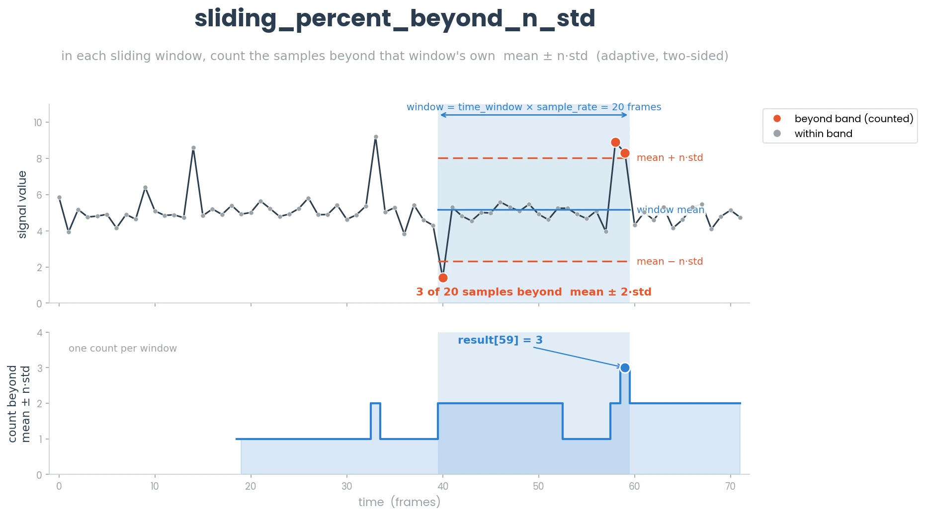
Parameters

• data (np.ndarray) – The input 1D data array for which the sliding window computation is to be performed.

• time_window (float) – The length of the time window in seconds.

• sample_rate (float) – The sample rate of the data in Hz (samples per second).

• value (float) – The number of standard deviations beyond which to count data points.

Returns

An array containing the count of data points beyond n standard deviations for each window.

Return type

np.ndarray

Example

>>> data = np.random.randint(0, 100, (100,))
>>> results = sliding_percent_beyond_n_std(data=data, time_window=1, sample_rate=10, value=2)

simba.data_processors.cuda.timeseries.sliding_spatial_density_cuda(x, radius, pixels_per_mm, window_size, sample_rate)

Computes the spatial density of points within a moving window along a trajectory using CUDA for acceleration.

This function calculates a spatial density measure for each point along a 2D trajectory path by counting the number of neighboring points within a specified radius. The computation is performed within a sliding window that moves along the trajectory, using GPU acceleration to handle large datasets efficiently.

EXPECTED RUNTIMES
FRAMES (MILLIONS)	GPU TIME (S)	GPU TIME (STEV)
2	0.5252	0.00063
4	1.0396	0.00099
8	2.0821	0.00231
16	4.2678	0.070249
32	8.4416	0.121225
64	16.941	0.097708
128	34.092	0.03986
256	68.052	0.27862
512	138.78118	3.755006
NVIDIA GeForce RTX 4070
time window = 2.5s @ 30 FPS
3 ITERATIONS

See also

simba.mixins.timeseries_features_mixin.TimeseriesFeatureMixin.spatial_density(), simba.mixins.timeseries_features_mixin.TimeseriesFeatureMixin.sliding_spatial_density()

Parameters

• x (np.ndarray) – A 2D array of shape (N, 2), where N is the number of points and each point has two spatial coordinates (x, y). The array represents the trajectory path of points in a 2D space (e.g., x and y positions in space).

• radius (float) – The radius (in millimeters) within which to count neighboring points around each trajectory point. Defines the area of interest around each point.

• pixels_per_mm (float) – The scaling factor that converts the physical radius (in millimeters) to pixel units for spatial density calculations.

• window_size (float) – The size of the sliding window (in seconds or points) to compute the density of points. A larger window size will consider more points in each density calculation.

• sample_rate (float) – The rate at which to sample the trajectory points (e.g., frames per second or samples per unit time). It adjusts the granularity of the sliding window.

Returns

A 1D numpy array where each element represents the computed spatial density for the trajectory at the corresponding point in time (or frame). Higher values indicate more densely packed points within the specified radius, while lower values suggest more sparsely distributed points.

Return type

np.ndarray

Example

>>> df = pd.read_csv("/mnt/c/troubleshooting/two_black_animals_14bp/project_folder/csv/outlier_corrected_movement_location/Test_3.csv")
>>> x = df[['Nose_1_x', 'Nose_1_y']].values
>>> results_cuda = sliding_spatial_density_cuda(x=x, radius=10.0, pixels_per_mm=4.0, window_size=1, sample_rate=20)

simba.data_processors.cuda.timeseries.sliding_threshold(data, time_window, sample_rate, value, inverse=False)

Compute the count of observations above or below threshold crossings over a sliding window using GPU acceleration.

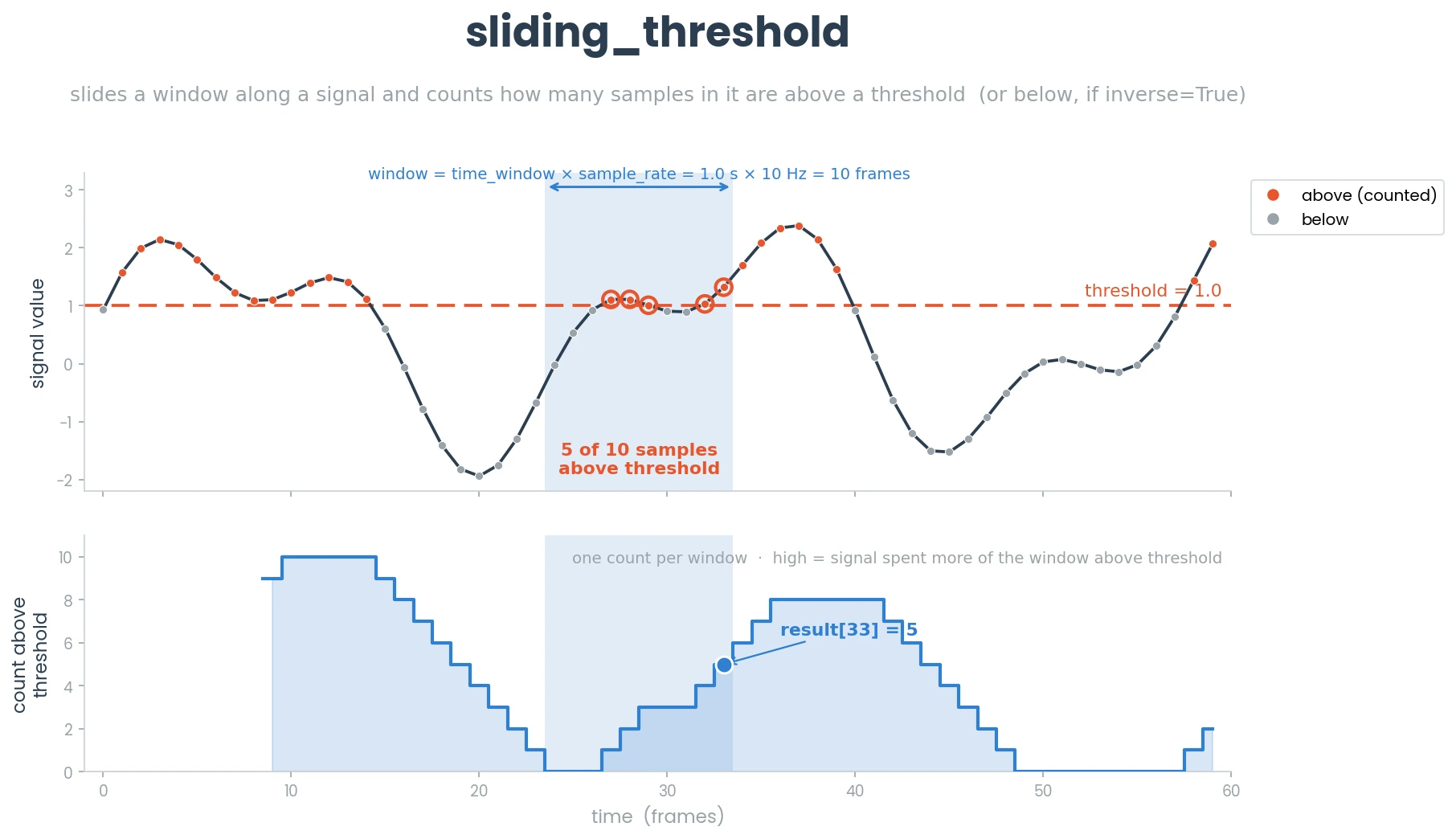
Parameters

• data (np.ndarray) – Input data array.

• time_window (float) – Size of the sliding window in seconds.

• sample_rate (float) – Number of samples per second in the data.

• value (float) – Threshold value.

• inverse (Optional[bool]) – If False, counts values above the threshold. If True, counts values below.

Returns

Array containing count of threshold crossings per window.

Return type

np.ndarray

SHAP explanations (GPU)

simba.data_processors.cuda.create_shap_log.create_shap_log(rf_clf, x, y, cnt_present, cnt_absent, x_names=None, clf_name=None, save_dir=None, verbose=True)

Computes SHAP (SHapley Additive exPlanations) values using a GPU for a RandomForestClassifier, based on specified counts of positive and negative samples, and optionally saves the results.

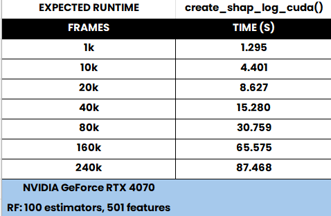
Note

1. The SHAP library has to be built from git repo rather than pip: pip install git+https://github.com/slundberg/shap.git.

2. The scikit model cannot be built using max_depth > 31. You can set this in the SimBA config under [create ensemble settings][rf_max_depth], or rf_max_depth in the config CSV’s.

Parameters

• rf_clf (Union[str, os.PathLike, RandomForestClassifier]) – Trained RandomForestClassifier model or path to the saved model. Can be a string, os.PathLike object, or an instance of RandomForestClassifier.

• x (Union[pd.DataFrame, np.ndarray]) – Input features used for SHAP value computation. Can be a pandas DataFrame or numpy ndarray.

• y (Union[pd.DataFrame, pd.Series, np.ndarray]) – Target labels corresponding to the input features. Can be a pandas DataFrame, pandas Series, or numpy ndarray with 0 and 1 values.

• cnt_present (int) – Number of positive samples (label=1) to include in the SHAP value computation.

• cnt_absent (int) – Number of negative samples (label=0) to include in the SHAP value computation.

• x_names (Optional[List[str]]) – Optional list of feature names corresponding to the columns in x. If x is a DataFrame, this is extracted automatically.

• clf_name (Optional[str]) – Optional name for the classifier, used in naming output files. If not provided, it is extracted from the y labels if possible.

• save_dir (Optional[Union[str, os.PathLike]]) – Optional directory path where the SHAP values and corresponding raw features are saved as CSV files.

• verbose (Optional[bool]) – Optional boolean flag indicating whether to print progress messages. Defaults to True.

Return Union[None, Tuple[pd.DataFrame, pd.DataFrame, int]]

If save_dir is None, returns a tuple containing: - V: DataFrame with SHAP values, expected value, sum of SHAP values, prediction probability, and target labels. - R: DataFrame containing the raw feature values for the selected samples. - expected_value: The expected value from the SHAP explainer.

If save_dir is provided, the function returns None and saves the output to CSV files in the specified directory.

Example

>>> x = np.random.random((1000, 501)).astype(np.float32)
>>> y = np.random.randint(0, 2, size=(len(x), 1)).astype(np.int32)
>>> clf_names = [str(x) for x in range(501)]
>>> results = create_shap_log(rf_clf=MODEL_PATH, x=x, y=y, cnt_present=int(i/2), cnt_absent=int(i/2), clf_name='TEST', x_names=clf_names, verbose=False)

Data transformations (GPU)

simba.data_processors.cuda.data.egocentrically_align_pose_cuda(data, anchor_1_idx, anchor_2_idx, anchor_location, direction, batch_size=1000000)

Aligns a set of 2D points egocentrically based on two anchor points and a target direction using GPU acceleration.

Rotates and translates a 3D array of 2D points (e.g., time-series of frame-wise data) such that one anchor point is aligned to a specified location, and the direction between the two anchors is aligned to a target angle.

See also

For numpy function, see simba.utils.data.egocentrically_align_pose(). For numba alternative, see simba.utils.data.egocentrically_align_pose_numba(). To align both pose and video, see simba.data_processors.egocentric_aligner.EgocentricalAligner(). To egocentrically rotate video, see simba.video_processors.egocentric_video_rotator.EgocentricVideoRotator()

EXPECTED RUNTIMES
FRAMES (MILLIONS)	CUDA TIME (S)	CUDA TIME (STEV)
0.25	0.1882001	0.15372434
0.5	0.1221498	0.00574819
1	0.24	0.0307
2	0.38	0.1092
4	0.505	0.01590969
8	1.037	0.0346
16	3.42	1.53194867
7 BODY-PARTS PER FRAME
3 ITERATIONS
batch size 16M
DIDN’T TEST HIGHER N AS I DON’T HAVE THE NON-GPU RAM

Parameters

• data (np.ndarray) – A 3D array of shape (num_frames, num_points, 2) containing 2D points for each frame. Each frame is represented as a 2D array of shape (num_points, 2), where each row corresponds to a point’s (x, y) coordinates.

• anchor_1_idx (int) – The index of the first anchor point in data used as the center of alignment. This body-part will be placed in the center of the image.

• anchor_2_idx (int) – The index of the second anchor point in data used to calculate the direction vector. This bosy-part will be located direction degrees from the anchor_1 body-part.

• direction (int) – The target direction in degrees to which the vector between the two anchors will be aligned.

• anchor_location (np.ndarray) – A 1D array of shape (2,) specifying the target (x, y) location for anchor_1_idx after alignment.

• batch_size (int) – Size of data that is processed on each iteration on GPU. default 1m. Increase if GPU allows.

Returns

A tuple containing the rotated data, and variables required for also rotating the video using the same rules: - aligned_data: A 3D array of shape (num_frames, num_points, 2) with the aligned 2D points. - centers: A 2D array of shape (num_frames, 2) containing the original locations of anchor_1_idx in each frame before alignment. - rotation_vectors: A 3D array of shape (num_frames, 2, 2) containing the rotation matrices applied to each frame.

Return type

Tuple[np.ndarray, np.ndarray, np.ndarray]

Example

>>> DATA_PATH = r"/mnt/c/Users/sroni/OneDrive/Desktop/rotate_ex/data/501_MA142_Gi_Saline_0513.csv"
>>> VIDEO_PATH = r"/mnt/c/Users/sroni/OneDrive/Desktop/rotate_ex/videos/501_MA142_Gi_Saline_0513.mp4"
>>> SAVE_PATH = r"/mnt/c/Users/sroni/OneDrive/Desktop/rotate_ex/videos/501_MA142_Gi_Saline_0513_rotated.mp4"
>>> ANCHOR_LOC = np.array([300, 300])
>>>
>>> df = read_df(file_path=DATA_PATH, file_type='csv')
>>> bp_cols = [x for x in df.columns if not x.endswith('_p')]
>>> data = df[bp_cols].values.reshape(len(df), int(len(bp_cols)/2), 2).astype(np.int64)
>>> data, centers, rotation_matrices = egocentrically_align_pose_cuda(data=data, anchor_1_idx=6, anchor_2_idx=2, anchor_location=ANCHOR_LOC, direction=180,batch_size=36000000)

GPU utilities

Low-level CUDA device primitives (@cuda.jit(device=True)) that the other GPU kernels compose, plus the public NVDEC video-decoder factory.

Low-level CUDA/Numba GPU helpers.

This module holds the small @cuda.jit(device=True) primitives (means, medians, standard deviation, MAD, RMS, ranges, Euclidean distance, matrix multiply/transpose, RGB-to-grey conversions and NaN-aware reductions) that the other simba.data_processors.cuda kernels compose, together with the public get_nvc_decoder() factory for GPU (NVDEC) hardware video decoding.

How to use

The _cuda_* functions are CUDA device functions: they execute on the GPU and can only be called from inside another CUDA kernel (a function decorated with @cuda.jit) or another device function — never directly from host/Python code. They operate on data already resident in GPU memory (device arrays, or thread-local scratch arrays), take one element/row per thread, and return plain scalars or arrays for further use inside the kernel. Call them as ordinary functions within a kernel; Numba inlines them at compile time (there is no kernel-launch overhead per call).

from numba import cuda
from simba.data_processors.cuda.utils import _cuda_mean, _cuda_std

@cuda.jit
def zscore_rows(data, out):           # data: (n_rows, row_len) device array
    i = cuda.grid(1)
    if i < data.shape[0]:
        row = data[i]
        m = _cuda_mean(row)           # device helpers, called from within the kernel
        s = _cuda_std(row, m)
        out[i] = (row[0] - m) / s

zscore_rows[blocks, threads](d_data, d_out)   # launch on device arrays

Notes:

• The reductions backed by a fixed thread-local scratch buffer (_cuda_mac(), _cuda_mad(), _cuda_rms(), _cuda_abs_energy()) assume inputs of at most 512 elements.

• Several helpers mutate their argument in place (e.g. _cuda_bubble_sort(), _cuda_median(), _cuda_subtract_2d()) — pass a copy if you need the input preserved.

• The only host-callable entry point is get_nvc_decoder(), which builds an NVDEC hardware video decoder from ordinary Python code.

simba.data_processors.cuda.utils._cross_test(x, y, x1, y1, x2, y2)

Device: which side of a directed segment a point lies on (2D cross-product sign).

Parameters

• x (float) – X-coordinate of the test point.

• y (float) – Y-coordinate of the test point.

• x1 (float) – X-coordinate of the segment start.

• y1 (float) – Y-coordinate of the segment start.

• x2 (float) – X-coordinate of the segment end.

• y2 (float) – Y-coordinate of the segment end.

Returns

True if the point lies to the right of the directed segment (x1,y1)->(x2,y2).

simba.data_processors.cuda.utils._cuda_2d_transpose(x, y)

Device: transpose a 2D array.

Parameters

• x (np.ndarray) – Input 2D array of shape (m, n).

• y (np.ndarray) – Output 2D array of shape (n, m) that receives the transpose.

Returns

The output array y.

simba.data_processors.cuda.utils._cuda_abs_energy(x)

Device: absolute energy (sum of squared elements) of a 1D array.

Parameters

x (np.ndarray) – Input 1D array (maximum length 512).

Returns

Sum of the squared elements of x.

simba.data_processors.cuda.utils._cuda_add_2d(x, vals)

Device: add a per-column 1D vector to every row of a 2D array (in place).

Parameters

• x (np.ndarray) – Input 2D array, modified in place.

• vals (np.ndarray) – 1D array with one value per column of x.

Returns

The modified array x.

simba.data_processors.cuda.utils._cuda_are_rows_equal(x, y, idx_1, idx_2)

Device: check whether a row in one 2D array equals a row in another.

Parameters

• x (np.ndarray) – First 2D array.

• y (np.ndarray) – Second 2D array (same number of columns as x).

• idx_1 (int) – Row index into x.

• idx_2 (int) – Row index into y.

Returns

True if row idx_1 of x equals row idx_2 of y.

simba.data_processors.cuda.utils._cuda_bubble_sort(x)

Device: in-place bubble sort of a 1D array (ascending).

Parameters

x (np.ndarray) – Input 1D array, sorted in place.

Returns

The sorted array x.

simba.data_processors.cuda.utils._cuda_cos(x, t)

Device: element-wise cosine of x written into t.

Parameters

• x (np.ndarray) – Input 1D array of angles in radians.

• t (np.ndarray) – Output 1D array (same length as x) that receives the cosines.

Returns

The output array t.

simba.data_processors.cuda.utils._cuda_diff(x, start, end, diff)

Compute first-order differences of a slice of x and store in diff.

Parameters

• x (np.ndarray) – Input array.

• start (int) – Start index (inclusive) of the slice

• end (int) – End index (exclusive) of the slice.

• diff (np.ndarray) – Output array to store differences of x[start:end].

Example

>>> diff = cuda.local.array(shape=512, dtype=float64)  # pre-allocated local array
>>> cuda_diff(x, 0, 5, diff)

simba.data_processors.cuda.utils._cuda_digital_pixel_to_grey(r, g, b)

Device: Rec.601 digital greyscale value of an RGB pixel.

Parameters

• r (int) – Red channel value.

• g (int) – Green channel value.

• b (int) – Blue channel value.

Returns

Greyscale (Rec.601 digital) value of the pixel.

simba.data_processors.cuda.utils._cuda_luminance_pixel_to_grey(r, g, b)

Device: Rec.709 luminance greyscale value of an RGB pixel.

Parameters

• r (int) – Red channel value.

• g (int) – Green channel value.

• b (int) – Blue channel value.

Returns

Greyscale (Rec.709 luminance) value of the pixel.

simba.data_processors.cuda.utils._cuda_mac(x)

Device: mean absolute change (mean of |x[i] - x[i-1]|) of a 1D array.

Parameters

x (np.ndarray) – Input 1D array (maximum length 512).

Returns

Mean of the absolute first-order differences of x.

simba.data_processors.cuda.utils._cuda_mad(x)

Device: median absolute deviation (MAD) of a 1D array.

Parameters

x (np.ndarray) – Input 1D array (maximum length 512).

Returns

Median absolute deviation of x.

simba.data_processors.cuda.utils._cuda_matrix_multiplication(mA, mB, out)

Device: matrix multiplication mA @ mB accumulated into out.

Parameters

• mA (np.ndarray) – Left 2D matrix of shape (m, k).

• mB (np.ndarray) – Right 2D matrix of shape (k, n).

• out (np.ndarray) – Pre-zeroed output 2D matrix of shape (m, n) that receives the product.

Returns

The output matrix out.

simba.data_processors.cuda.utils._cuda_max(x)

Device: maximum value of a 1D array.

Parameters

x (np.ndarray) – Input 1D array.

Returns

Largest element of x.

simba.data_processors.cuda.utils._cuda_mean(x)

Device: arithmetic mean of a 1D array.

Parameters

x (np.ndarray) – Input 1D array.

Returns

Mean of x.

simba.data_processors.cuda.utils._cuda_median(x)

Device: median of a 1D array.

Parameters

x (np.ndarray) – Input 1D array (sorted in place as a side effect).

Returns

Median value of x.

simba.data_processors.cuda.utils._cuda_min(x)

Device: minimum value of a 1D array.

Parameters

x (np.ndarray) – Input 1D array.

Returns

Smallest element of x.

simba.data_processors.cuda.utils._cuda_mse(img_1, img_2)

Device: mean squared error between two equally-shaped 2D images.

Parameters

• img_1 (np.ndarray) – First 2D image.

• img_2 (np.ndarray) – Second 2D image (same shape as img_1).

Returns

Mean squared error between the two images.

simba.data_processors.cuda.utils._cuda_nanmean(x, N)

Compute the mean of x ignoring NaN values.

Parameters

• x (np.ndarray) – Input array of length N.

• N (int) – Number of elements in x to consider.

Returns

Mean of non-NaN elements in x. Returns 0.0 if no valid elements found.

simba.data_processors.cuda.utils._cuda_nanvariance(x, N)

Compute the variance of x ignoring NaN values using the unbiased estimator.

Parameters

• x (np.ndarray) – Input array of length N.

• N (int) – Number of elements in x to consider. Note this is

Returns

Variance of non-NaN elements in x. Returns 0.0 if count <= 1.

simba.data_processors.cuda.utils._cuda_range(x)

Device: range (max minus min) of a 1D array.

Parameters

x (np.ndarray) – Input 1D array.

Returns

Difference between the maximum and minimum of x.

simba.data_processors.cuda.utils._cuda_rms(x)

Device: root-mean-square of a 1D array.

Parameters

x (np.ndarray) – Input 1D array (maximum length 512).

Returns

Root-mean-square of x.

simba.data_processors.cuda.utils._cuda_sin(x, t)

Device: element-wise sine of x written into t.

Parameters

• x (np.ndarray) – Input 1D array of angles in radians.

• t (np.ndarray) – Output 1D array (same length as x) that receives the sines.

Returns

The output array t.

simba.data_processors.cuda.utils._cuda_standard_deviation(x)

Device: population standard deviation of a 1D array (divides by N).

Parameters

x (np.ndarray) – Input 1D array.

Returns

Standard deviation of x.

simba.data_processors.cuda.utils._cuda_std(x, x_hat)

Device: standard deviation of x about a precomputed mean.

Parameters

• x (np.ndarray) – Input 1D array.

• x_hat (float) – Precomputed mean of x.

Returns

Standard deviation of x about x_hat.

simba.data_processors.cuda.utils._cuda_subtract_2d(x, vals)

Device: subtract a per-column 1D vector from every row of a 2D array (in place).

Parameters

• x (np.ndarray) – Input 2D array, modified in place.

• vals (np.ndarray) – 1D array with one value per column of x.

Returns

The modified array x.

simba.data_processors.cuda.utils._cuda_sum(x)

Device: sum of a 1D array.

Parameters

x (np.ndarray) – Input 1D array.

Returns

Sum of all elements of x.

simba.data_processors.cuda.utils._cuda_variance(x)

Device: sample variance of a 1D array (divides by N-1).

Parameters

x (np.ndarray) – Input 1D array.

Returns

Variance of x.

simba.data_processors.cuda.utils._deg2rad(x)

Device: convert an angle from degrees to radians.

Parameters

x (float) – Angle in degrees.

Returns

Angle in radians.

simba.data_processors.cuda.utils._euclid_dist_2d(x, y)

Device: Euclidean distance between two 2D points.

Parameters

• x (np.ndarray) – First point as a length-2 array (x, y).

• y (np.ndarray) – Second point as a length-2 array (x, y).

Returns

Euclidean distance between the two points.

simba.data_processors.cuda.utils._is_cuda_available()

Check if GPU available. If True, returns the GPUs, the model, physical slots and compute capabilitie(s).

Returns

Two-part tuple with first value indicating with the GPU is available (bool) and the second value denoting GPU attributes (dict).

Return type

Tuple[bool, Dict[int, Any]]

simba.data_processors.cuda.utils._rad2deg(x)

Device: convert an angle from radians to degrees.

Parameters

x (float) – Angle in radians.

Returns

Angle in degrees.

simba.data_processors.cuda.utils.get_nvc_decoder(video_path, output_color_type, gpu_id=0, use_device_memory=False)

Create an NVDEC hardware video decoder for GPU-accelerated frame reading.

Parameters

• video_path (Union[str, os.PathLike]) – Path to the video file to decode.

• output_color_type – PyNvVideoCodec output colour format for decoded frames.

• gpu_id (int) – Index of the GPU to decode on. Default 0.

• use_device_memory (bool) – If True, keep decoded frames in GPU device memory; otherwise copy to host.

Raises

SimBAGPUError – If PyNvVideoCodec is not installed, or if no CUDA GPU is available.

Returns

A configured PyNvVideoCodec.SimpleDecoder.