Statistics transformations

Statistics mixin

class simba.mixins.statistics_mixin.Statistics

Statistics methods used for feature extraction, drift assessment, distance computations, distribution comparisons in sliding and static windows.

Note

Most methods implemented using numba parallelization for improved run-times. See line graph below for expected run-times for a few methods included in this class.

Most method has numba typed signatures to decrease compilation time through reduced type inference. Make sure to pass the correct dtypes as indicated by signature decorators. If dtype is not specified at array creation, it will typically be float64 or int64. As most methods here use float32 for the input data argument, make sure to downcast.

This class contains a few probability distribution comparison methods. These are being moved to simba.sandbox.distances (05.24).

References

1

Bernard Desgraupes - https://cran.r-project.org/web/packages/clusterCrit/vignettes/clusterCrit.pdf

2

Ikotun, A. M., Habyarimana, F., & Ezugwu, A. E. (2025). Cluster validity indices for automatic clustering: A comprehensive review. Heliyon, 11(2), e41953. https://doi.org/10.1016/j.heliyon.2025.e41953

3

Hassan, B. A., Tayfor, N. B., Hassan, A. A., Ahmed, A. M., Rashid, T. A., & Abdalla, N. N. (2024). From A-to-Z review of clustering validation indices. arXiv. https://doi.org/10.48550/arXiv.2407.20246

4

Leland McInnes - pynndescent.

static adjusted_mutual_info(x, y)

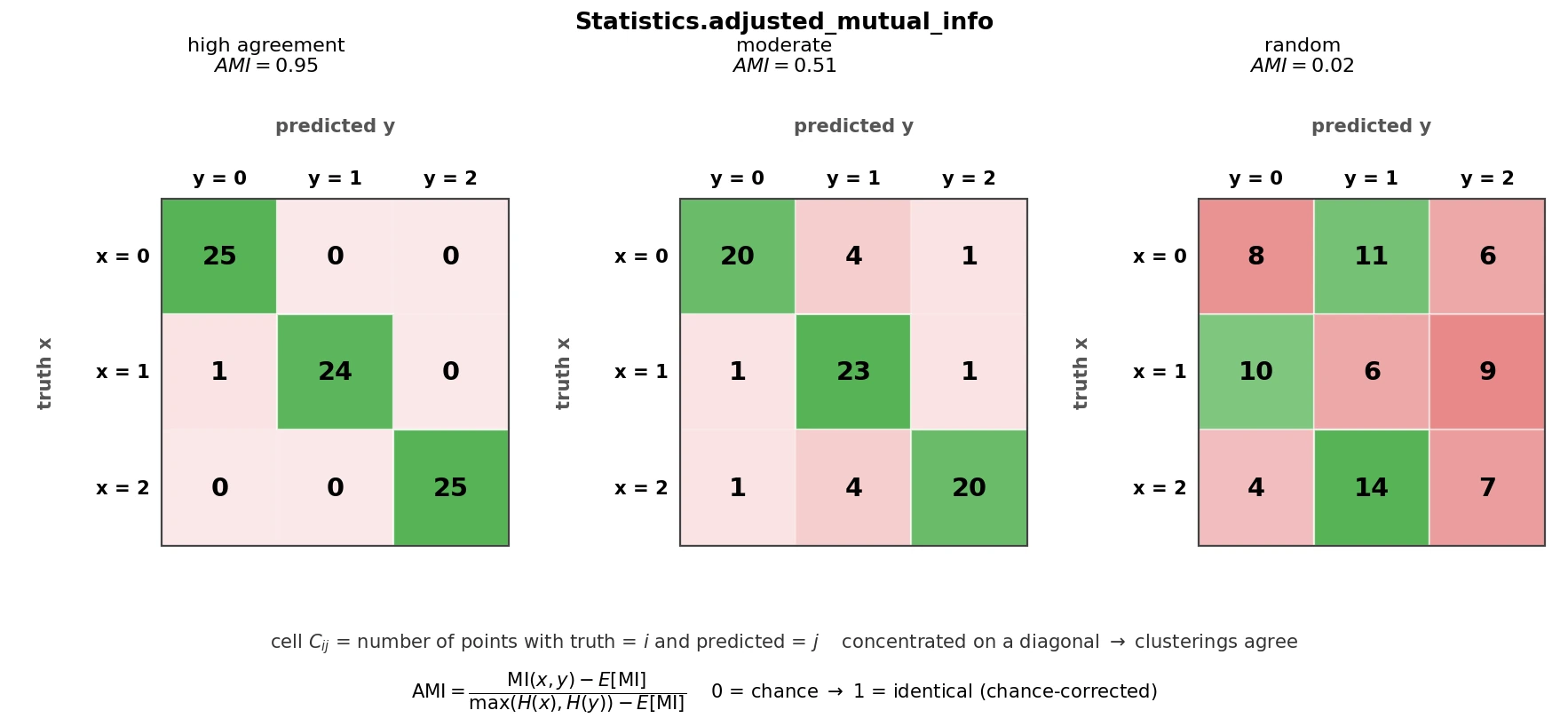
Calculate the Adjusted Mutual Information (AMI) between two clusterings as a measure of similarity.

Calculates the Adjusted Mutual Information (AMI) between two sets of cluster labels. AMI measures the agreement between two clustering results, accounting for chance agreement. The value of AMI ranges from 0 (indicating no agreement) to 1 (perfect agreement).

\[\mathrm{AMI}(x, y) = \frac{\mathrm{MI}(x, y) - E(\mathrm{MI}(x, y))}{\max(H(x), H(y)) - E(\mathrm{MI}(x, y))}\]

where:

• \(\text{MI}(x, y)\) is the mutual information between \(x\) and \(y\).

• \(E(\text{MI}(x, y))\) is the expected mutual information.

• \(H(x)\) and \(H(y)\) are the entropies of \(x\) and \(y\), respectively.

Parameters

• x (np.ndarray) – 1D array representing the labels of the first model.

• y (np.ndarray) – 1D array representing the labels of the second model.

Returns

Score between 0 and 1, where 1 indicates perfect clustering agreement.

Return type

float

static adjusted_rand(x, y)

Calculate the Adjusted Rand Index (ARI) between two clusterings.

The Adjusted Rand Index (ARI) is a measure of the similarity between two clusterings. It considers all pairs of samples and counts pairs that are assigned to the same or different clusters in both the true and predicted clusterings.

The ARI is defined as:

\[ARI = \frac{TP + TN}{TP + FP + FN + TN}\]

where:

• \(TP\) (True Positive) is the number of pairs of elements that are in the same cluster in both x and y,

• \(FP\) (False Positive) is the number of pairs of elements that are in the same cluster in y but not in x,

• \(FN\) (False Negative) is the number of pairs of elements that are in the same cluster in x but not in y,

• \(TN\) (True Negative) is the number of pairs of elements that are in different clusters in both x and y.

The ARI value ranges from -1 to 1. A value of 1 indicates perfect clustering agreement, 0 indicates random clustering, and negative values indicate disagreement between the clusterings.

Note

Modified from scikit-learn

See also

For GPU call, see simba.data_processors.cuda.statistics.adjusted_rand_gpu()

Parameters

• x (np.ndarray) – 1D array representing the labels of the first model.

• y (np.ndarray) – 1D array representing the labels of the second model.

Returns

A value of 1 indicates perfect clustering agreement, a value of 0 indicates random clustering, and negative values indicate disagreement between the clusterings.

Return type

float

Example

>>> x = np.array([0, 0, 0, 0, 0])
>>> y = np.array([1, 1, 1, 1, 1])
>>> Statistics.adjusted_rand(x=x, y=y)
>>> 1.0

static banfeld_raftery_index(x, y)

Computes the Banfeld-Raftery index for clustering evaluation.

Smaller values represent better clustering. Values can be negative.

Parameters

• x – 2D NumPy array of shape (n_samples, n_features) representing the dataset.

• y – 1D NumPy array of shape (n_samples,) containing cluster labels for each data point.

Returns

The Banfeld-Raftery index.

Return type

float

References

1

Banfield, J. D., & Raftery, A. E. (1993). Model-based Gaussian and non-Gaussian clustering. Biometrics, 49(3), 803-821. https://doi.org/10.2307/2532201

static bouguessa_wang_sun_v2(x, y)

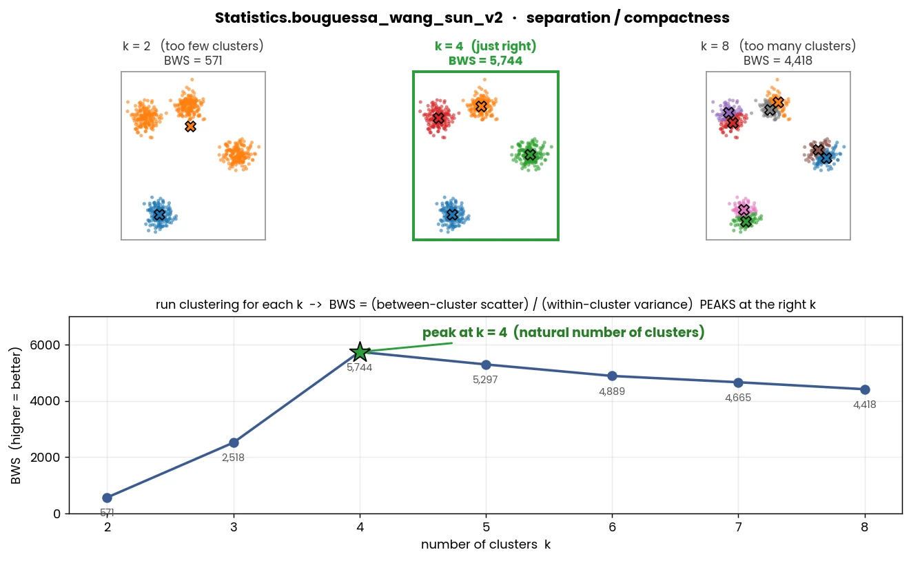
Compute the Bouguessa-Wang-Sun (BWS) index using covariance matrices and means.

Parameters

• x (np.ndarray) – A 2D array of shape (n_samples, n_features) representing the feature vectors of the data points.

• y (np.ndarray) – A 1D array of shape (n_samples,) containing the cluster labels for each data point.

Returns

The BWS index value (between-cluster scatter / total within-cluster variance). Higher values indicate better clustering.

Return type

float

Example

>>> from sklearn.datasets import make_blobs
>>> X, y = make_blobs(n_samples=500, centers=3, random_state=42)
>>> Statistics.bouguessa_wang_sun_v2(X, y)

References

1

Bouguessa, M., Wang, S., & Sun, H. (2006). An objective approach to cluster validation. Pattern Recognition Letters, 27(13), 1419–1430.

static bray_curtis_dissimilarity(x, w=None)

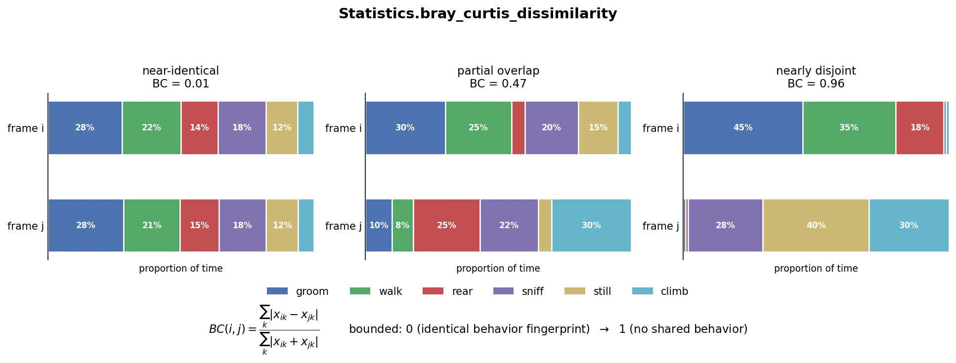
Jitted compute of the Bray-Curtis dissimilarity matrix between samples based on feature values.

The Bray-Curtis dissimilarity measures the dissimilarity between two samples based on their feature values. It is useful for finding similar frames based on behavior.

Useful for finding similar frames based on behavior.

Note

Adapted from pynndescent.

Parameters

• x (np.ndarray) – 2d array with likely normalized feature values.

• w (Optional[np.ndarray]) – Optional 2d array with weights of same size as x. Default None and all observations will have the same weight.

Returns

2d array with same size as x representing dissimilarity values. 0 and the observations are identical and at 1 the observations are completly disimilar.

Return type

np.ndarray

Example

>>> x = np.array([[1, 1, 1, 1, 1], [0, 0, 0, 0, 0], [0, 0, 0, 0, 0], [1, 1, 1, 1, 1]]).astype(np.float32)
>>> Statistics().bray_curtis_dissimilarity(x=x)
>>> [[0, 1., 1., 0.], [1., 0., 0., 1.], [1., 0., 0., 1.], [0., 1., 1., 0.]]

static brunner_munzel(sample_1, sample_2)

Jitted compute of Brunner-Munzel W between two distributions.

The Brunner-Munzel W statistic compares the central tendency and the spread of two independent samples. It is useful for comparing the distribution of a continuous variable between two groups, especially when the assumptions of parametric tests like the t-test are violated.

Note

Modified from scipy.stats.brunnermunzel

\[W = -\frac{n_x \cdot n_y \cdot (\bar{R}_y - \bar{R}_x)}{(n_x + n_y) \cdot \sqrt{n_x \cdot S_x + n_y \cdot S_y}}\]

where:

• \(n_x\) and \(n_y\) are the sizes of sample_1 and sample_2 respectively,

• \(\bar{R}_x\) and \(\bar{R}_y\) are the mean ranks of sample_1 and sample_2, respectively.

• \(S_x\) and \(S_y\) are the dispersion statistics of sample_1 and sample_2 respectively.

Parameters

• sample_1 (np.ndarray) – First 1d array representing feature values.

• sample_2 (np.ndarray) – Second 1d array representing feature values.

Returns

Brunner-Munzel W statistic.

Return type

float

Example

>>> sample_1, sample_2 = np.random.normal(loc=10, scale=2, size=10), np.random.normal(loc=20, scale=2, size=10)
>>> Statistics().brunner_munzel(sample_1=sample_1, sample_2=sample_2)
0.5751408161437165

static c_index(x, y)

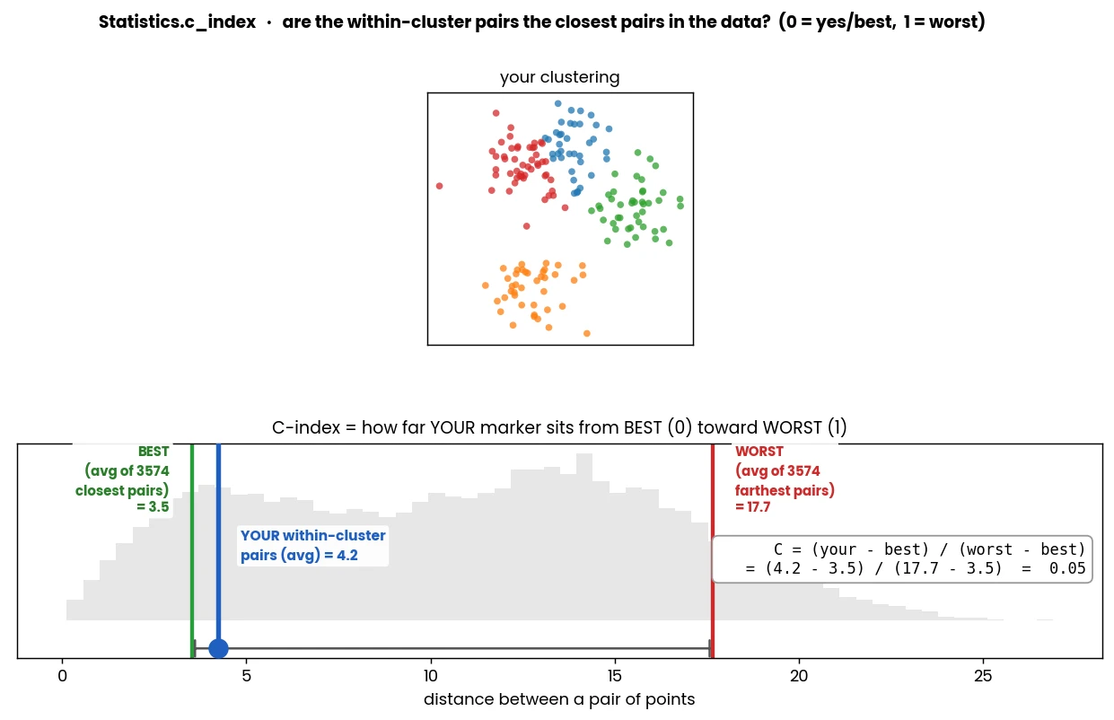
Calculate the C Index for clustering evaluation.

Parameters

• x (np.ndarray) – A 2D array of shape (n_samples, n_features) containing the data points.

• y (np.ndarray) – A 1D array of shape (n_samples,) containing cluster labels for the data points.

Returns

The C Index value, ranging from 0 to 1.

Return type

float

The C Index ranges from 0 to 1:

• 0 indicates perfect clustering (clusters are as compact as possible).

• 1 indicates worst clustering (clusters are highly spread out).

References

1

Hubert, L. J., & Levin, J. R. (1976). A general statistical framework for assessing categorical clustering in free recall. Psychological Bulletin, 83(6), 1072–1080.

Example

>>> X, y = make_blobs(n_samples=800, centers=2, n_features=3, random_state=0, cluster_std=0.1)
>>> Statistics.c_index(x=X, y=y)

static calinski_harabasz(x, y)

Compute the Calinski-Harabasz score to evaluate clustering quality.

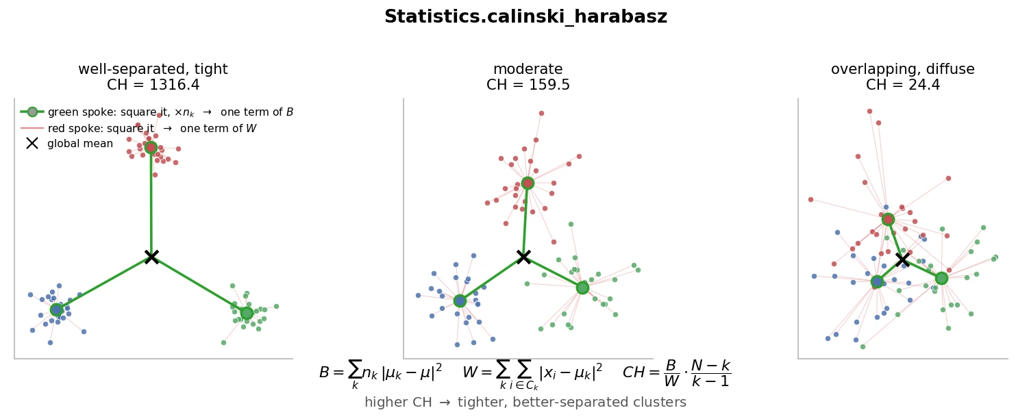
The Calinski-Harabasz score is a measure of cluster separation and compactness. It is calculated as the ratio of the between-cluster dispersion to the within-cluster dispersion. A higher score indicates better clustering.

Note

Modified from scikit-learn

The Calinski-Harabasz score (CH) is calculated as:

\[CH = \frac{B}{W} \times \frac{N - k}{k - 1}\]

where: - \(B\) is the sum of squared distances between cluster centroids, - \(W\) is the sum of squared distances from each point to its assigned cluster centroid, - \(N\) is the total number of data points, - \(k\) is the number of clusters.

Parameters

• x – 2D array representing the data points. Shape (n_samples, n_features/n_dimension).

• y – 2D array representing cluster labels for each data point. Shape (n_samples,).

Returns

Calinski-Harabasz score.

Float

float

Example

Example

>>> x = np.random.random((100, 2)).astype(np.float32)
>>> y = np.random.randint(0, 100, (100,)).astype(np.int64)
>>> Statistics.calinski_harabasz(x=x, y=y)

static chi_square(sample_1, sample_2, critical_values=None, type='goodness_of_fit')

Jitted compute of chi square between two categorical distributions.

Note

Requires sample_1 and sample_2 has to be numeric. if working with strings, convert to numeric category values before using chi_square.

Warning

Non-overlapping values (i.e., categories exist in sample_1 that does not exist in sample2) or small values may cause inflated chi square values. If small contingency table small values, consider TODO Fisher’s exact test

Parameters

• sample_1 (ndarray) – First 1d array representing feature values.

• sample_2 (ndarray) – Second 1d array representing feature values.

• critical_values (ndarray) – 2D array with where indexes represent degrees of freedom and values represent critical values. Can be found in simba.assets.critical_values_05.pickle

Returns

Size-2 tuple with the chi-square value and significance threshold boolean (if critical_values is not None).

Return type

Tuple[float, Union[bool, None]]

Example

>>> sample_1 = np.array([1, 1, 2, 2, 3, 3, 4, 4, 5, 5, 5]).astype(np.float32)
>>> sample_2 = np.array([1, 2, 3, 4, 5, 6, 7, 8, 9, 10]).astype(np.float32)
>>> critical_values = pickle.load(open("simba/assets/lookups/critical_values_5.pickle", "rb"))['chi_square']['one_tail'].values
>>> Statistics.chi_square(sample_1=sample_2, sample_2=sample_1, critical_values=critical_values, type='goodness_of_fit')
>>> (8.333, False)
>>>

chow_test()

static circular_euclidean_kantorovich(x, y)

Compute the circular Euclidean Kantorovich (Wasserstein) distance between two discrete distributions.

Suitable for comparing distributions of circular data such as angles, time-of-day, phase etc.

Param

np.ndarray x: 1D array representing the first discrete distribution or histogram.

Param

np.ndarray x: 1D array representing the second discrete distribution or histogram.

Note

Distance metric: smaller values represent similar distributions. Adapted from pynndescent.

Example

>>> x, y = np.random.normal(loc=65, scale=10, size=10000000), np.random.normal(loc=90, scale=1, size=10000000)
>>> b =Statistics.circular_euclidean_kantorovich(x, y)

static cochrans_q(data)

Compute Cochrans Q for 2-dimensional boolean array.

Cochran’s Q statistic is used to test for significant differences between more than two proportions. It can be used to evaluate if the performance of multiple (>=2) classifiers on the same data is the same or significantly different.

Note

If two classifiers, consider simba.mixins.statistics.Statistics.mcnemar().

Useful background: https://psych.unl.edu/psycrs/handcomp/hccochran.PDF

\(Q = \frac{(k - 1) \left( kG^2 - \left( \sum_{j=1}^{k} C_j \right)^2 \right)}{kR - S}\)

where:

• \(k\) is the number of classifiers,

• \(G = \sum_{j=1}^{k} C_j^2\) (the sum of the squares of the column sums),

• \(C_j\) is the sum of the \(j\)-th column (number of successes for the \(j\)-th classifier),

• \(R = \sum_{i=1}^{n} R_i\) (the total number of successes across all classifiers),

• \(S = \sum_{i=1}^{n} R_i^2\) (the sum of the squares of the row sums),

• \(R_i\) is the sum of the \(i\)-th row (number of successes for the \(i\)-th observation).

Parameters

data (np.ndarray) – Two-dimensional array of boolean values where axis 1 represents classifiers or features and rows represent frames.

Returns

Cochran’s Q statistic signidicance value.

Return type

Tuple[float, float]

Example

>>> data = np.random.randint(0, 2, (100000, 4))
>>> Statistics.cochrans_q(data=data)

static cohens_d(sample_1, sample_2)

Jitted compute of Cohen’s d between two distributions.

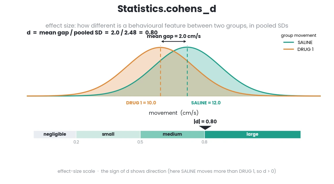
Cohen’s d is a measure of effect size that quantifies the difference between the means of two distributions in terms of their standard deviation. It is calculated as the difference between the means of the two distributions divided by the pooled standard deviation.

Higher values indicate a larger effect size, with 0.2 considered a small effect, 0.5 a medium effect, and 0.8 or above a large effect. Negative values indicate that the mean of sample 2 is larger than the mean of sample 1.

See also

For time-series based method, see simba.mixins.statistics_mixin.Statistics.rolling_cohens_d()

\[d = \frac{\bar{x}_1 - \bar{x}_2}{\sqrt{\frac{s_1^2 + s_2^2}{2}}}\]

where:

• \(\bar{x}_1\) and \(\bar{x}_2\) are the means of sample_1 and sample_2 respectively,

• \(s_1\) and \(s_2\) are the standard deviations of sample_1 and sample_2 respectively.

Parameters

• sample_1 (np.ndarray) – First 1d array representing feature values.

• sample_2 (np.ndarray) – Second 1d array representing feature values.

Returns

Cohen’s D statistic.

Return type

float

Example

>>> sample_1 = [2, 4, 7, 3, 7, 35, 8, 9]
>>> sample_2 = [4, 8, 14, 6, 14, 70, 16, 18]
>>> Statistics().cohens_d(sample_1=sample_1, sample_2=sample_2)
-0.5952099775170546

static cohens_h(sample_1, sample_2)

Jitted compute Cohen’s h effect size for two samples of binary [0, 1] values. Cohen’s h is a measure of effect size for comparing two independent samples based on the differences in proportions of the two samples.

Note

Modified from DABEST Cohen’s h wiki

\[\text{Cohen's h} = 2 \arcsin\left(\sqrt{\frac{\sum\text{sample\_1}}{N\_1}}\right) - 2 \arcsin\left(\sqrt{\frac{\sum\text{sample\_2}}{N\_2}}\right)\]

Where \(N_1\) and \(N_2\) are the sample sizes of sample_1 and sample_2, respectively.

Parameters

• sample_1 (np.ndarray) – 1D array with binary [0, 1] values (e.g., first classifier inference values).

• sample_2 (np.ndarray) – 1D array with binary [0, 1] values (e.g., second classifier inference values).

Returns

Cohen’s h effect size.

Return type

float

Example

>>> sample_1 = np.array([1, 0, 0, 1])
>>> sample_2 = np.array([1, 1, 1, 0])
>>> Statistics().cohens_h(sample_1=sample_1, sample_2=sample_2)
>>> -0.5235987755982985

static cohens_kappa(sample_1, sample_2)

Jitted compute Cohen’s Kappa coefficient for two binary samples.

Cohen’s Kappa coefficient measures the agreement between two sets of binary ratings, taking into account agreement occurring by chance. It ranges from -1 to 1, where 1 indicates perfect agreement, 0 indicates agreement by chance, and -1 indicates complete disagreement.

\[\kappa = 1 - \frac{\sum{w_{ij} \cdot D_{ij}}}{\sum{w_{ij} \cdot E_{ij}}}\]

where:

• \(\kappa\) is Cohen’s Kappa coefficient,

• \(w_{ij}\) are the weights,

• \(D_{ij}\) are the observed frequencies,

• \(E_{ij}\) are the expected frequencies.

Parameters

• sample_1 (np.ndarray) – The first binary sample, a 1D NumPy array of integers.

• sample_2 (np.ndarray) – The second binary sample, a 1D NumPy array of integers.

Returns

Cohen’s Kappa coefficient between the two samples.

Return type

float

Example

>>> sample_1 = np.random.randint(0, 2, size=(10000,))
>>> sample_2 = np.random.randint(0, 2, size=(10000,))
>>> Statistics.cohens_kappa(sample_1=sample_1, sample_2=sample_2))

static concordance_ratio(x, invert)

Calculate the concordance ratio of a 2D numpy array. The concordance ratio is a measure of agreement in a dataset. It is calculated as the ratio of the number of rows that contain only one unique value to the total number of rows.

The equation for the concordance ratio \(C\) is given by:

\[C = \frac{N_c}{N_t}\]

where:

• \(N_c\) is the count of rows with only one unique value,

• \(N_t\) is the total number of rows in the array.

If the invert parameter is set to True, the function will return the disconcordance ratio instead, defined as:

\[D = \frac{N_d}{N_t}\]

where:

• \(N_d\) is the count of rows with more than one unique value.

Parameters

• x (np.ndarray) – A 2D numpy array with ordinals represented as integers.

• invert (bool) – If True, the concordance ratio is inverted, and disconcordance ratio is returned

Returns

The concordance ratio, representing the count of rows with only one unique value divided by the total number of rows in the array.

Return type

float

Example

>>> x = np.random.randint(0, 2, (5000, 4))
>>> results = Statistics.concordance_ratio(x=x, invert=False)

static cop_index(x, y, epsilon=1e-16)

Computes the Clustering Overall Performance (COP) Index for evaluating clustering quality.

The COP Index is defined as the ratio of the average intra-cluster compactness (C) to the average inter-cluster separation (S). A lower COP index indicates better clustering, as it implies tight clusters and greater separation between them.

Parameters

• x (np.ndarray) – A 2D array of shape (n_samples, n_features) representing the feature vectors of the data points.

• y (np.ndarray) – A 1D array of shape (n_samples,) containing the cluster labels for each data point.

Returns

The COP index value. Lower values indicate better clustering.

Return type

float

References

1

Gurrutxaga, I., Albisua, I., Arbelaitz, O., Martín, J. I., Muguerza, J., Pérez, J. M., & Perona, I. (2011). SEP/COP: an efficient method to find the best partition in hierarchical clustering based on a new cluster validity index. Pattern Recognition, 44(4), 810–820.

Example

>>> X, y = make_blobs(n_samples=50000, centers=10, n_features=3, random_state=0, cluster_std=1)
>>> Statistics.cop_index(x=X, y=y)

static cov_matrix(data)

Jitted helper to compute the covariance matrix of the input data. Helper for computing cronbach alpha, multivariate analysis, and distance computations.

Parameters

data (np.ndarray) – 2-dimensional numpy array representing the input data with shape (n, m), where n is the number of observations and m is the number of features.

Returns

Covariance matrix of the input data with shape (m, m). The (i, j)-th element of the matrix represents the covariance between the i-th and j-th features in the data.

Example

>>> data = np.random.randint(0,2, (200, 40)).astype(np.float32)
>>> covariance_matrix = Statistics.cov_matrix(data=data)

static czebyshev_distance(sample_1, sample_2)

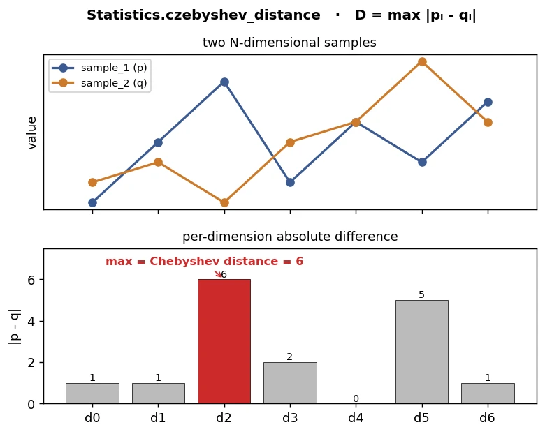
Calculate the Czebyshev distance between two N-dimensional samples.

The Czebyshev distance is defined as the maximum absolute difference between the corresponding elements of the two arrays.

Note

Normalize arrays sample_1 and sample_2 before passing it to ensure accurate results.

The equation for the Czebyshev distance is given by \(D_\infty(p, q) = \max_i \left| p_i - q_i \right|\).

See also

simba.mixins.statistics_mixin.Statistics.sliding_czebyshev_distance()

Parameters

• sample_1 (np.ndarray) – The first sample, an N-dimensional NumPy array.

• sample_2 (np.ndarray) – The second sample, an N-dimensional NumPy array.

Return float

The Czebyshev distance between the two samples.

Example

>>> sample_1 = np.random.randint(0, 10, (10000,100))
>>> sample_2 = np.random.randint(0, 10, (10000,100))
>>> Statistics.czebyshev_distance(sample_1=sample_1, sample_2=sample_2)

static d_prime(x, y, lower_limit=0.0001, upper_limit=0.9999)

Computes d-prime from two Boolean 1d arrays, e.g., between classifications and ground truth.

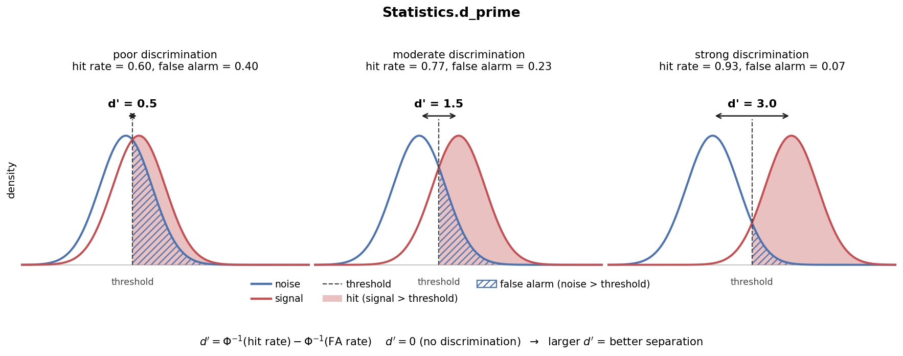
D-prime (d’) is a measure of signal detection performance, indicating the ability to discriminate between signal and noise. It is computed as the difference between the inverse cumulative distribution function (CDF) of the hit rate and the false alarm rate.

\[d' = \Phi^{-1}(hit\_rate) - \Phi^{-1}(false\_alarm\_rate)\]

where: - \(\Phi^{-1}\) is the inverse of the cumulative distribution function (CDF) of the normal distribution, - \(hit\_rate\) is the proportion of true positives correctly identified, - \(false\_alarm\_rate\) is the proportion of false positives incorrectly identified.

Parameters

• x (np.ndarray) – Boolean 1D array of response values, where 1 represents presence, and 0 representing absence.

• y (np.ndarray) – Boolean 1D array of ground truth, where 1 represents presence, and 0 representing absence.

• lower_limit (Optional[float]) – Lower limit to bound hit and false alarm rates. Defaults to 0.0001.

• upper_limit (Optional[float]) – Upper limit to bound hit and false alarm rates. Defaults to 0.9999.

Returns

The calculated d’ (d-prime) value.

Return type

float

Example

>>> x = np.random.randint(0, 2, (1000,))
>>> y = np.random.randint(0, 2, (1000,))
>>> Statistics.d_prime(x=x, y=y)

davis_bouldin(x, y)

Calculate the Davis-Bouldin index for evaluating clustering performance.

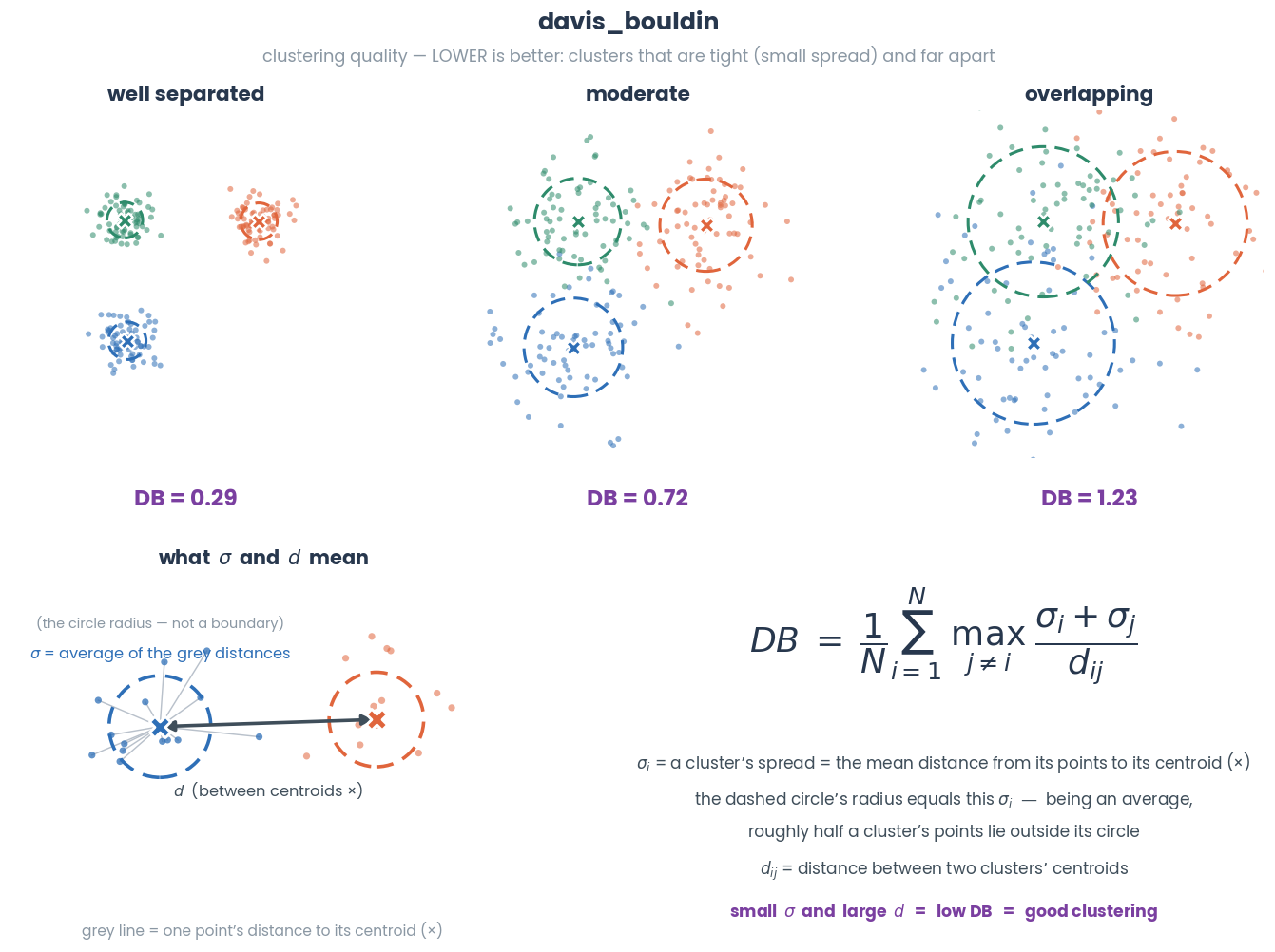
Davis-Bouldin index measures the clustering quality based on the within-cluster similarity and between-cluster dissimilarity. Lower values indicate better clustering.

See also

For GPU acceleration, use simba.data_processors.cuda.statistics.davis_bouldin()

Note

Modified from scikit-learn

\[DB = \frac{1}{N} \sum_{i=1}^{N} \max_{j \neq i} \left( \frac{\sigma_i + \sigma_j}{d_{ij}} \right)\]

where: - \(N\) is the number of clusters, - \(\sigma_i\) is the average distance between each point in cluster \(i\) and the centroid of cluster \(i\), - \(d_{ij}\) is the distance between the centroids of clusters \(i\) and \(j\).

Parameters

• x (np.ndarray) – 2D array representing the data points. Shape (n_samples, n_features/n_dimension).

• y (np.ndarray) – 2D array representing cluster labels for each data point. Shape (n_samples,).

Returns

Davis-Bouldin score.

Return type

float

Example

>>> x = np.random.randint(0, 100, (100, 2))
>>> y = np.random.randint(0, 3, (100,))
>>> Statistics.davis_bouldin(x=x, y=y)

static dunn_index(x, y, sample=None)

Calculate the Dunn index to evaluate the quality of clustered labels.

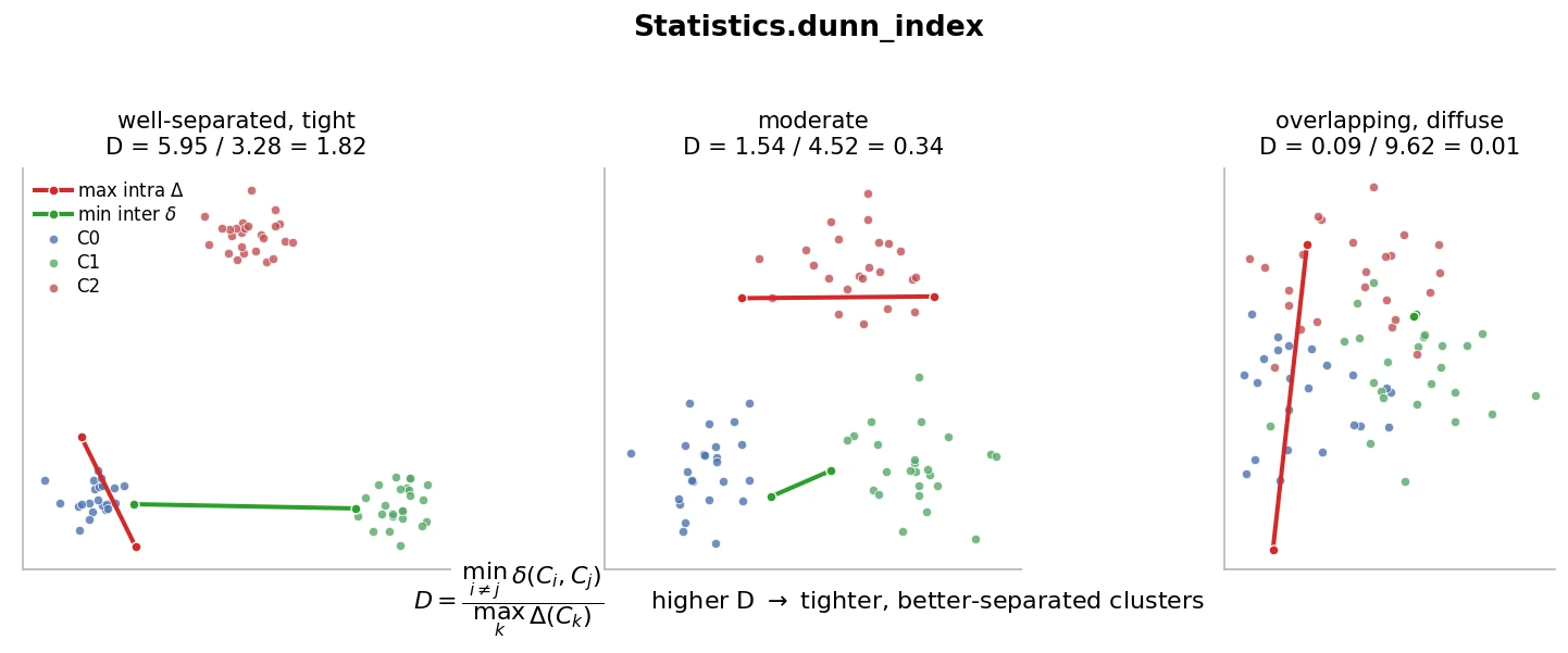
This function calculates the Dunn Index, which is a measure of clustering quality. The index considers the ratio of the minimum inter-cluster distance to the maximum intra-cluster distance. The Dunn Index range from zero to infinity and larger values indicate better clustering. The Dunn Index uses Euclidean distances.

The Dunn Index is calculated using the following steps:

1. Inter-cluster distance: Compute the distances between each pair of clusters and find the minimum distance.

2. Intra-cluster distance: Determine the distances within each cluster and find the maximum distance.

The Dunn Index is given by:

\[D = \frac{\min_{i \neq j} \{ \delta(C_i, C_j) \}}{\max_k \{ \Delta(C_k) \}}\]

where \(\delta(C_i, C_j)\) is the distance between clusters \(C_i\) and \(C_j\), and \(\Delta(C_k)\) is the diameter of cluster \(C_k\).

Note

Modified from jqmviegas

Wiki https://en.wikipedia.org/wiki/Dunn_index

If Dunn Index can not be calculated, -1 is returned.

Note

For GPU accelerated method, use simba.data_processors.cuda.statistics.dunn_index().

Parameters

• x (np.ndarray) – 2D array representing the data points. Shape (n_samples, n_features).

• y (np.ndarray) – 1D array representing cluster labels for each data point. Shape (n_samples,).

Returns

The Dunn index value

Return type

float

Example

>>> x = np.random.randint(0, 100, (100, 2))
>>> y = np.random.randint(0, 3, (100,))
>>> Statistics.dunn_index(x=x, y=y)

static dunn_symmetry_idx(x, y)

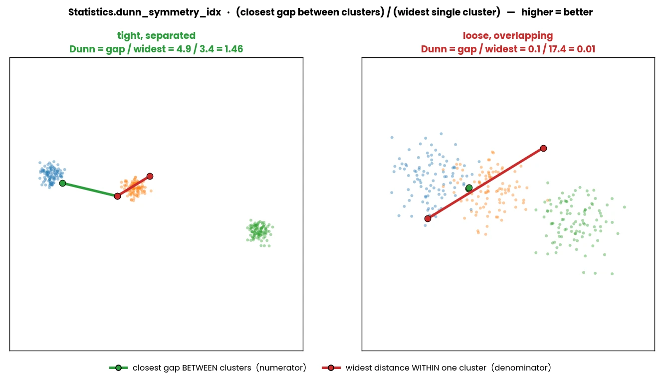
DunnSym index output range positive real numbers 0 -> ∞ where 0 is extremely poor clustering and higher values represent better cluster separation.

Parameters

• x – 2D array representing the data points. Shape (n_samples, n_features/n_dimension).

• y – 2D array representing cluster labels for each data point. Shape (n_samples,).

Return float

Dynn-Symmetry index.

References

1

Ikotun, A. M., Habyarimana, F., & Ezugwu, A. E. (2025). Cluster validity indices for automatic clustering: A comprehensive review. Heliyon, 11(2), e41953. https://doi.org/10.1016/j.heliyon.2025.e41953

2

Hassan, B. A., Tayfor, N. B., Hassan, A. A., Ahmed, A. M., Rashid, T. A., & Abdalla, N. N. (2024). From A-to-Z review of clustering validation indices. arXiv. https://doi.org/10.48550/arXiv.2407.20246

Example

>>> x, y = make_blobs(n_samples=1000, n_features=2, centers=5, random_state=42, cluster_std=0.1)
>>> Statistics.dunn_symmetry_idx(x=x, y=y)

static elliptic_envelope(data, contamination=0.1, normalize=False, groupby_idx=None)

Compute the Mahalanobis distances of each observation in the input array using Elliptic Envelope method.

Parameters

• data – Input data array of shape (n_samples, n_features).

• contamination (Optional[float]) – The proportion of outliers to be assumed in the data. Defaults to 0.1.

• normalize (Optional[bool]) – Whether to normalize the Mahalanobis distances between 0 and 1. Defaults to True.

Returns

The Mahalanobis distances of each observation in array. Larger values indicate outliers.

Return type

np.ndarray

Example

>>> data, lbls = make_blobs(n_samples=2000, n_features=2, centers=1, random_state=42)
>>> envelope_score = elliptic_envelope(data=data, normalize=True)
>>> results = np.hstack((data[:, 0:2], envelope_score.reshape(lof.shape[0], 1)))
>>> results = pd.DataFrame(results, columns=['X', 'Y', 'ENVELOPE SCORE'])
>>> PlottingMixin.continuous_scatter(data=results, palette='seismic', bg_clr='lightgrey', columns=['X', 'Y', 'ENVELOPE SCORE'],size=30)

static eta_squared(x, y)

Calculate eta-squared, a measure of between-subjects effect size.

Eta-squared (\(\eta^2\)) is calculated as the ratio of the sum of squares between groups to the total sum of squares. Range from 0 to 1, where larger values indicate a stronger effect size.

The equation for eta squared is defined as: \(\eta^2 = \frac{SS_{between}}{SS_{between} + SS_{within}}\)

where:

• \(SS_{between}\) is the sum of squares between groups,

• \(SS_{within}\) is the sum of squares within groups.

See also

For sliding time-windows comparisons, see simba.mixins.statistics_mixin.Statistics.sliding_eta_squared().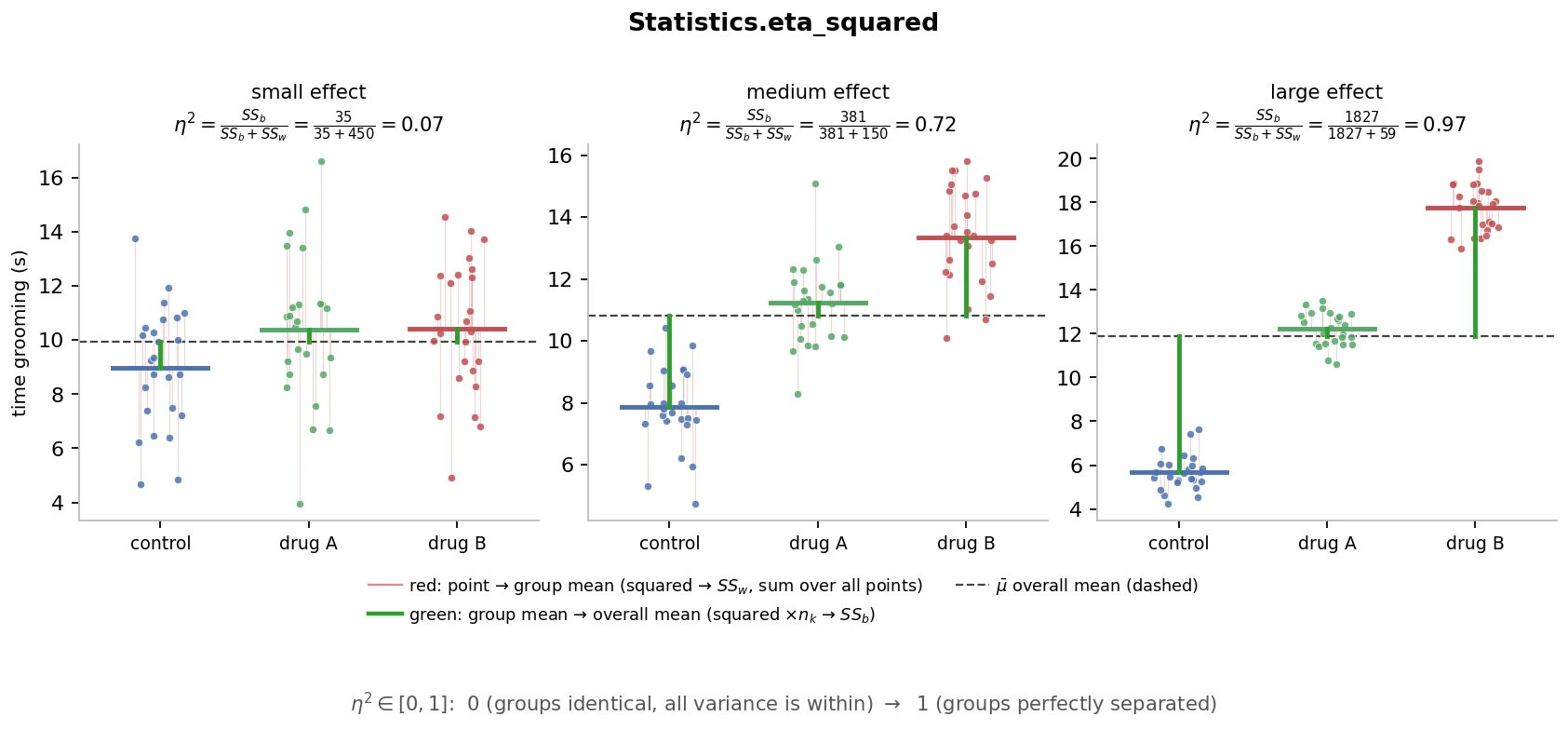

Parameters

• x (np.ndarray) – 1D array containing the dependent variable data.

• y (np.ndarray) – 1d array containing the grouping variable (categorical) data of same size as x.

Returns

The eta-squared value representing the proportion of variance in the dependent variable that is attributable to the grouping variable.

Return type

float

static find_collinear_features(df, threshold, method='pearson', verbose=False)

Identify collinear features in the dataframe based on the specified correlation method and threshold.

See also

For multicore numba accelerated method, see simba.mixins.train_model_mixin.TrainModelMixin.find_highly_correlated_fields().

Parameters

• df (pd.DataFrame) – Input DataFrame containing features.

• threshold (float) – Threshold value to determine collinearity.

• method (Optional[Literal['pearson', 'spearman', 'kendall']]) – Method for calculating correlation. Defaults to ‘pearson’.

Returns

Set of feature names identified as collinear. Returns one feature for every feature pair with correlation value above specified threshold.

Return type

List[str]

Example

>>> x = pd.DataFrame(np.random.randint(0, 100, (100, 100)))
>>> names = Statistics.find_collinear_features(df=x, threshold=0.2, method='pearson', verbose=True)

static fowlkes_mallows(x, y)

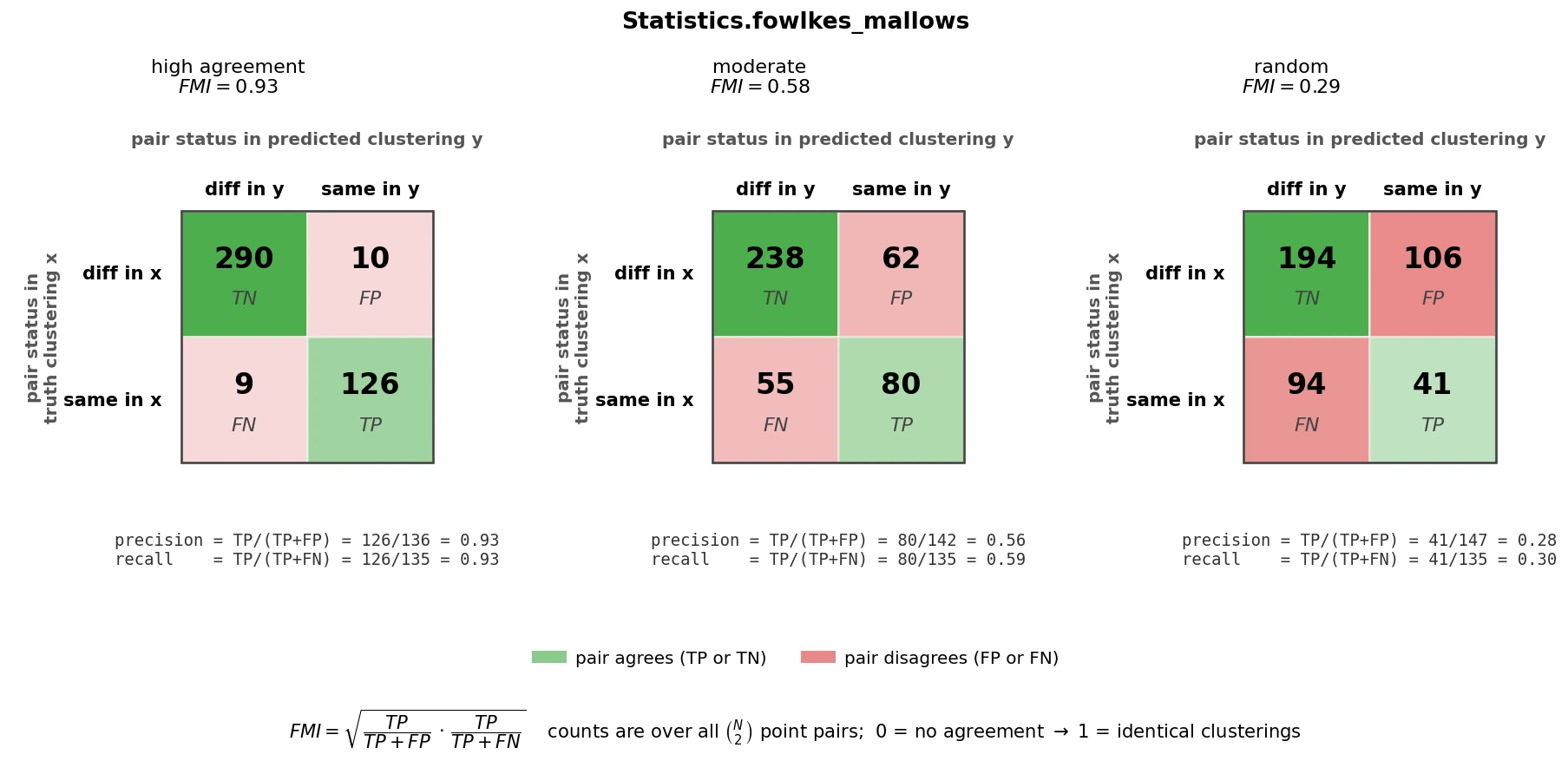
Calculate the Fowlkes-Mallows Index (FMI) between two clusterings.

The Fowlkes-Mallows index (FMI) is a measure of similarity between two clusterings. It compares the similarity of the clusters obtained by two different clustering algorithms or procedures.

The index is defined as the geometric mean of the pairwise precision and recall:

\[FMI = \sqrt{\frac{TP}{TP + FP} \times \frac{TP}{TP + FN}}\]

where: - \(TP\) (True Positive) is the number of pairs of elements that are in the same cluster in both x and y, - \(FP\) (False Positive) is the number of pairs of elements that are in the same cluster in y but not in x, - \(FN\) (False Negative) is the number of pairs of elements that are in the same cluster in x but not in y.

Note

Modified from scikit-learn

Parameters

• x (np.ndarray) – 1D array representing the labels of the first model.

• y (np.ndarray) – 1D array representing the labels of the second model.

Return float

Score between 0 and 1. 1 indicates perfect clustering agreement, 0 indicates random clustering.

static geometric_mean(x)

Computes the geometric mean of a 1D NumPy array.

Parameters

x – A 1D NumPy array of numeric type containing non-negative values. Must have at least two elements.

Returns

The geometric mean of the values in x.

Return type

float

static get_clustering_purity(x, y)

Compute clustering quality using purity score.

An external evaluation metric for clustering quality. It measures the extent to which clusters contain a single class. The score ranges from 0 to 1, where 1 indicates perfect purity.

Note

Adapted from Ugurite’s Stack Overflow answer: https://stackoverflow.com/a/51672699

Parameters

• x (np.ndarray) – Predicted cluster labels (1D array of integers).

• y (np.ndarray) – Ground truth class labels (1D array of integers, same length as x).

Returns

Purity score in the range [0, 1].

Return type

float

Example

>>> x = np.random.randint(0, 5, (100000,))
>>> y = np.random.randint(0, 4, (100000,))
>>> p = Statistics.get_clustering_purity(x=x, y=y)

References

1

Evaluation of clustering. Introduction to Information Retrieval. Available at: https://nlp.stanford.edu/IR-book/html/htmledition/evaluation-of-clustering-1.html

static gower_distance(x, y)

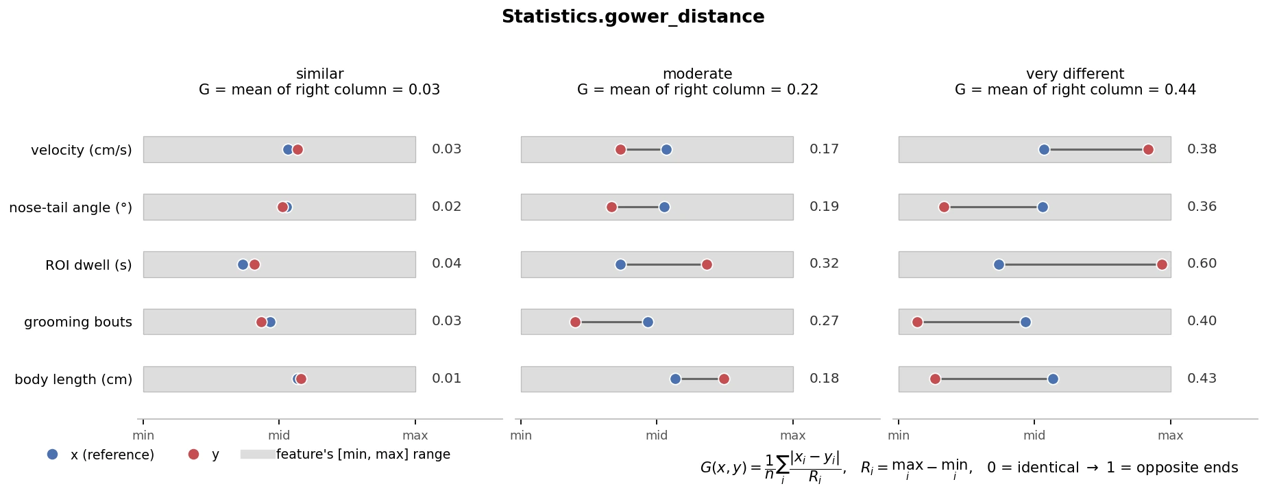
Compute Gower-like distance vector between corresponding rows of two numerical matrices. Gower distance is a measure of dissimilarity between two vectors (or rows in this case).

Note

This function assumes x and y have the same shape and only considers numerical attributes.

Each observation in x is compared to the corresponding observation in y based on normalized absolute differences across numerical columns.

Parameters

• x (np.ndarray) – First numerical matrix with shape (m, n).

• y (np.ndarray) – Second numerical matrix with shape (m, n).

Returns

Gower-like distance vector with shape (m,).

Return type

np.ndarray

Example

>>> x, y = np.random.randint(0, 500, (1000, 6000)), np.random.randint(0, 500, (1000, 6000))
>>> Statistics.gower_distance(x=x, y=y)

References

1

Gower, J. C. (1971). A general coefficient of similarity and some of its properties. Biometrics, 27(4), 857–874. https://doi.org/10.2307/2528823

static grubbs_test(x, left_tail=False)

Perform Grubbs’ test to detect outliers if the minimum or maximum value in a feature series is an outlier.

Grubbs’ test is a statistical test used to detect outliers in a univariate data set. It calculates the Grubbs’ test statistic as the absolute difference between the extreme value (either the minimum or maximum) and the sample mean, divided by the sample standard deviation.

\[\text{Grubbs' Test Statistic} = \frac{|\bar{x} - x_{\text{min/max}}|}{s}\]

where:

• \(\bar{x}\) is the sample mean,

• \(x_{\text{min/max}}\) is the minimum or maximum value of the sample (depending on the tail being tested),

• \(s\) is the sample standard deviation.

Parameters

• x (np.ndarray) – 1D array representing numeric data.

• left_tail (Optional[bool]) – If True, the test calculates the Grubbs’ test statistic for the left tail (minimum value). If False (default), it calculates the statistic for the right tail (maximum value).

Returns

The computed Grubbs’ test statistic.

Return type

float

Example

>>> x = np.random.random((100,))
>>> Statistics.grubbs_test(x=x)

static hamming_distance(x, y, sort=False, w=None)

Jitted compute of the Hamming similarity between two vectors.

The Hamming similarity measures the similarity between two binary vectors by counting the number of positions at which the corresponding elements are different.

Note

If w is not provided, equal weights are assumed. Adapted from pynndescent.

\[\text{Hamming distance}(x, y) = \frac{{\sum_{i=1}^{n} w_i}}{{n}}\]

where:

• \(n\) is the length of the vectors,

• \(w_i\) is the weight associated with the math:`i`th element of the vectors.

See also

For GPU method, see simba.data_processors.cuda.statistics.hamming_distance_gpu().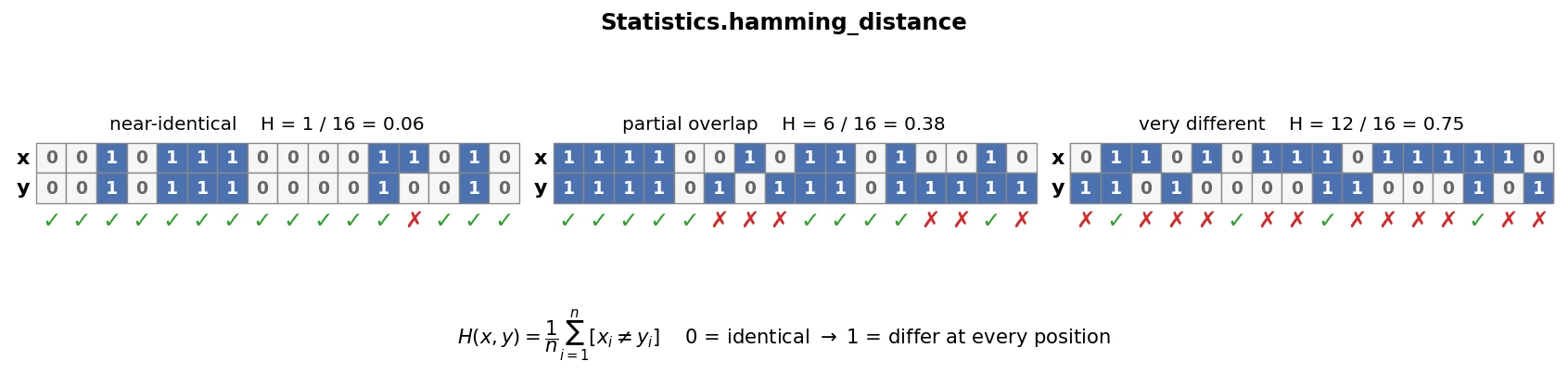

Parameters

• x (np.ndarray) – First binary vector.

• y (np.ndarray) – Second binary vector.

• w (Optional[np.ndarray]) – Optional weights for each element. Can be classification probabilities. If not provided, equal weights are assumed.

• sort (Optional[bool]) – If True, sorts x and y prior to hamming distance calculation. Default, False.

Returns

Hamming similarity

Return type

float

Example

>>> x, y = np.random.randint(0, 2, (10,)).astype(np.int8), np.random.randint(0, 2, (10,)).astype(np.int8)
>>> Statistics().hamming_distance(x=x, y=y)
>>> 0.91

static hartley_fmax(x, y)

Compute Hartley’s Fmax statistic to test for equality of variances between two features or groups.

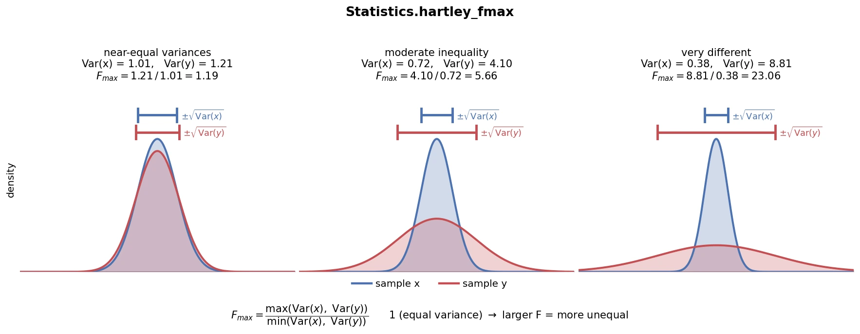
Hartley’s Fmax statistic is used to test whether two samples have equal variances. It is calculated as the ratio of the largest sample variance to the smallest sample variance. Values close to one represent closer to equal variance.

\[\text{Hartley's } F_{max} = \frac{\max(\text{Var}(x), \text{Var}(y))}{\min(\text{Var}(x), \text{Var}(y))}\]

where: - \(\text{Var}(x)\) is the variance of sample \(x\), - \(\text{Var}(y)\) is the variance of sample \(y\).

Parameters

• x (np.ndarray) – 1D array representing numeric data of the first group/feature.

• y (np.ndarray) – 1D array representing numeric data of the second group/feature.

Returns

Hartley’s Fmax statistic.

Return type

float

Example

>>> x = np.random.random((100,))
>>> y = np.random.random((100,))
>>> Statistics.hartley_fmax(x=x, y=y)

hbos(data, bucket_method='auto')

Jitted compute of Histogram-based Outlier Scores (HBOS). HBOS quantifies the abnormality of data points based on the densities of their feature values within their respective buckets over all feature values.

Parameters

• data (np.ndarray) – 2d array with frames represented by rows and columns representing feature values.

• bucket_method (Literal) – Estimator determining optimal bucket count and bucket width. Default: The maximum of the Sturges and Freedman-Diaconis estimators.

Returns

Array of size data.shape[0] representing outlier scores, with higher values representing greater outliers.

Return type

np.ndarray

Example

>>> sample_1 = np.random.random_integers(low=1, high=2, size=(10, 50)).astype(np.float64)
>>> sample_2 = np.random.random_integers(low=7, high=20, size=(2, 50)).astype(np.float64)
>>> data = np.vstack([sample_1, sample_2])
>>> Statistics().hbos(data=data)

hellinger_distance(x, y, bucket_method='auto')

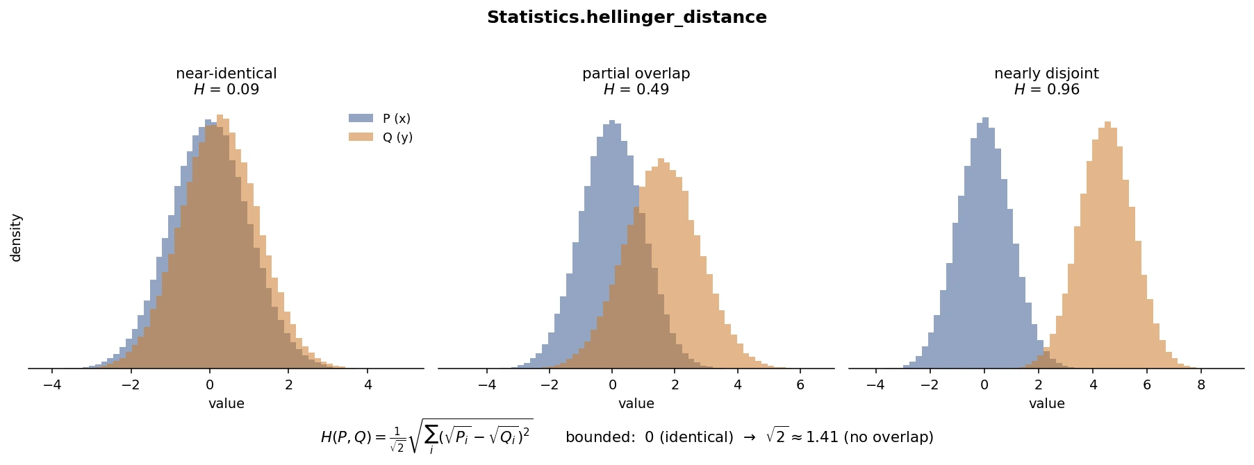
Compute the Hellinger distance between two vector distributions.

Note

The Hellinger distance is bounded and ranges from 0 to √2. Distance of √2 indicates that the two distributions are maximally dissimilar

\[H(P, Q) = \frac{1}{\sqrt{2}} \sqrt{ \sum_{i=1}^{n} (\sqrt{P(i)} - \sqrt{Q(i)})^2 }\]

where: - \(P(i)\) is the probability of the \(i\)-th event in distribution \(P\), - \(Q(i)\) is the probability of the \(i\)-th event in distribution \(Q\), - \(n\) is the number of events.

Parameters

• x (np.ndarray) – First 1D array representing a probability distribution.

• y (np.ndarray) – Second 1D array representing a probability distribution.

• bucket_method (Optional[Literal['fd', 'doane', 'auto', 'scott', 'stone', 'rice', 'sturges', 'sqrt']]) – Method for computing histogram bins. Default is ‘auto’.

Returns

Hellinger distance between the two input probability distributions.

Return type

float

Example

>>> x = np.random.randint(0, 9000, (500000,))
>>> y = np.random.randint(0, 9000, (500000,))
>>> Statistics().hellinger_distance(x=x, y=y, bucket_method='auto')

static i_index(x, y, verbose=False)

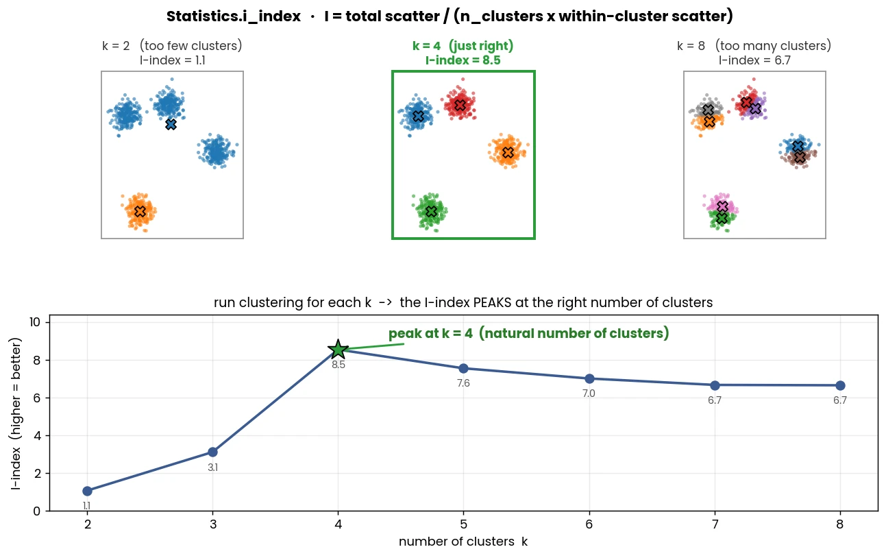
Calculate the I-Index for evaluating clustering quality.

The I-Index is a metric that measures the compactness and separation of clusters. A higher I-Index indicates better clustering with compact and well-separated clusters.

See also

To compute I-index on GPU, use i_index()

Parameters

• x (np.ndarray) – The dataset as a 2D NumPy array of shape (n_samples, n_features).

• y (np.ndarray) – Cluster labels for each data point as a 1D NumPy array of shape (n_samples,).

Returns

The I-index score for the dataset.

Return type

float

References

1

Zhao, Q., Xu, M., & Fränti, P. (2009). Sum-of-squares based cluster validity index and significance analysis. In Adaptive and Natural Computing Algorithms (ICANNGA 2009), Lecture Notes in Computer Science, vol. 5495. Springer.

Example

>>> X, y = make_blobs(n_samples=5000, centers=20, n_features=3, random_state=0, cluster_std=0.1)
>>> Statistics.i_index(x=X, y=y)

static independent_samples_t(sample_1, sample_2, critical_values=None)

Jitted compute independent-samples t-test statistic and boolean significance between two distributions.

Note

Critical values are stored in simba.assets.lookups.critical_values_**.pickle

The t-statistic for independent samples t-test is calculated using the following formula:

\[t = \frac{\bar{x}_1 - \bar{x}_2}{s_p \sqrt{\frac{1}{n_1} + \frac{1}{n_2}}}\]

where: - \(\bar{x}_1\) and \(\bar{x}_2\) are the means of the two samples, - \(s_p\) is the pooled standard deviation, - \(n_1\) and \(n_2\) are the sizes of the two samples.

See also

simba.mixins.statistics_mixin.Statistics.rolling_independent_sample_t()

Parameters

• sample_1 (ndarray) – First 1d array representing feature values.

• sample_2 (ndarray) – Second 1d array representing feature values.

• critical_values (ndarray) – 2d array where the first column represents degrees of freedom and second column represents critical values.

Return t_statistic, p_value

Size-2 tuple representing t-statistic and associated probability value. p_value is None if critical_values is None. Else True or False with True representing significant.

Return type

Tuple[float, Union[None, bool]]

Example

>>> sample_1 = np.array([1, 2, 3, 1, 3, 2, 1, 10, 8, 4, 10])
>>> sample_2 = np.array([2, 5, 10, 4, 8, 10, 7, 10, 7, 10, 10])
>>> Statistics().independent_samples_t(sample_1=sample_1, sample_2=sample_2)
>>> (-2.5266046804590183, None)
>>> critical_values = pickle.load(open("simba/assets/lookups/critical_values_05.pickle","rb"))['independent_t_test']['one_tail'].values
>>> Statistics().independent_samples_t(sample_1=sample_1, sample_2=sample_2, critical_values=critical_values)
>>> (-2.5266046804590183, True)

static isolation_forest(x, estimators=0.2, groupby_idx=None, normalize=False)

An implementation of the Isolation Forest algorithm for outlier detection.

Note

The isolation forest scores are negated. Thus, higher values indicate more atypical (outlier) data points.

Parameters

• x (np.ndarray) – 2-D array with feature values.

• estimators (Union[int, float]) – Number of splits. If the value is a float, then interpreted as the ratio of x shape.

• groupby_idx (Optional[int]) – If int, then the index 1 of data for which to group the data and compute LOF on each segment. E.g., can be field holding a cluster identifier.

• normalize (Optional[bool]) – Whether to normalize the outlier score between 0 and 1. Defaults to False.

Returns

2D array with the x, y and the isolation forest outlier score for each observation.

Return type

np.ndarray

Example

>>> x, lbls = make_blobs(n_samples=10000, n_features=2, centers=10, random_state=42)
>>> x = np.hstack((x, lbls.reshape(-1, 1)))
>>> scores = isolation_forest(x=x, estimators=10, normalize=True)
>>> results = np.hstack((x[:, 0:2], scores.reshape(scores.shape[0], 1)))
>>> results = pd.DataFrame(results, columns=['X', 'Y', 'ISOLATION SCORE'])
>>> PlottingMixin.continuous_scatter(data=results, palette='seismic', bg_clr='lightgrey', columns=['X', 'Y', 'ISOLATION SCORE'],size=30)

References

1

Liu, Fei Tony, Kai Ming Ting, and Zhi-Hua Zhou. “Isolation Forest.” In 2008 Eighth IEEE International Conference on Data Mining, 413–22. Pisa, Italy: IEEE, 2008. https://doi.org/10.1109/ICDM.2008.17.

static jaccard_distance(x, y)

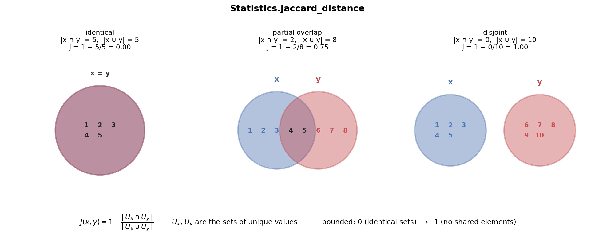
Calculate the Jaccard distance between two 1D NumPy arrays.

The Jaccard distance is a measure of dissimilarity between two sets. It is defined as the size of the intersection of the sets divided by the size of the union of the sets.

Parameters

• x (np.ndarray) – The first 1D NumPy array.

• y (np.ndarray) – The second 1D NumPy array.

Returns

The Jaccard distance between arrays x and y.

Return type

float

Example

>>> x = np.random.randint(0, 5, (100))
>>> y = np.random.randint(0, 7, (100))
>>> Statistics.jaccard_distance(x=x, y=y)
>>> 0.2857143

jensen_shannon_divergence(sample_1, sample_2, bucket_method='auto')

Compute Jensen-Shannon divergence between two distributions. Useful for (i) measure drift in datasets, and (ii) featurization of distribution shifts across sequential time-bins.

Note

JSD = 0: Indicates that the two distributions are identical. 0 < JSD < 1: Indicates a degree of dissimilarity between the distributions, with values closer to 1 indicating greater dissimilarity. JSD = 1: Indicates that the two distributions are maximally dissimilar.

\[JSD = \frac{KL(P_1 || M) + KL(P_2 || M)}{2}\]

See also

For rolling comparisons in a timeseries, see simba.mixins.statistics_mixin.Statistics.rolling_jensen_shannon_divergence()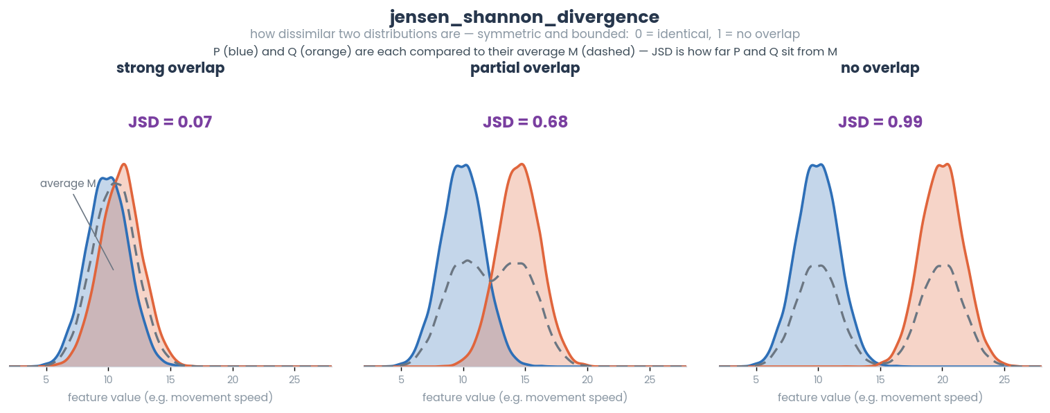

Parameters

• sample_1 (ndarray) – First 1d array representing feature values.

• sample_2 (ndarray) – Second 1d array representing feature values.

• bucket_method (Literal) – Estimator determining optimal bucket count and bucket width. Default: The maximum of the Sturges and Freedman-Diaconis estimators.

Returns

Jensen-Shannon divergence between sample_1 and sample_2

Return type

float

Example

>>> sample_1, sample_2 = np.array([1, 2, 3, 4, 5, 10, 1, 2, 3]), np.array([1, 5, 10, 9, 10, 1, 10, 6, 7])
>>> Statistics().jensen_shannon_divergence(sample_1=sample_1, sample_2=sample_2, bucket_method='fd')
>>> 0.3403  # 0 = identical distributions, 1 = maximally dissimilar (log base 2)

static kendall_tau(sample_1, sample_2)

Jitted compute of Kendall Tau (rank correlation coefficient). Non-parametric method for computing correlation between two time-series features. Returns tau and associated z-score.

Kendall Tau is a measure of the correspondence between two rankings. It compares the number of concordant pairs (pairs of elements that are in the same order in both rankings) to the number of discordant pairs (pairs of elements that are in different orders in the rankings).

Kendall Tau is calculated using the following formula:

\[\tau = \frac{{\sum C - \sum D}}{{\sum C + \sum D}}\]

where \(C\) is the count of concordant pairs and \(D\) is the count of discordant pairs.

See also

For time-series based comparison, see simba.mixins.statistics_mixin.Statistics.sliding_kendall_tau().

Parameters

• sample_1 (ndarray) – First 1D array with feature values.

• sample_2 (ndarray) – Second 1D array with feature values.

Returns

Size-2 tuple with Kendall Tau and associated z-score.

Return type

Tuple[float, float]

Examples

>>> sample_1 = np.array([4, 2, 3, 4, 5, 7]).astype(np.float32)
>>> sample_2 = np.array([1, 2, 3, 4, 5, 7]).astype(np.float32)
>>> Statistics().kendall_tau(sample_1=sample_1, sample_2=sample_2)
>>> (0.7333333333333333, 2.0665401605809928)

References

1

Stephanie Glen, “Kendall’s Tau (Kendall Rank Correlation Coefficient)”.

static kmeans_1d(data, k, max_iters, calc_medians)

Perform k-means clustering on a 1-dimensional dataset.

Note

• If calc_medians is True, the function returns cluster medians in addition to centroids and labels.

See also

Use with brighness intensity output to detect cue lights on/off states. Brighness intensity in images can be obtained using simba.mixins.image_mixin.ImageMixin.brightness_intensity(), or simba.data_processors.cuda.image.img_stack_brightness() for GPU acceleration.

Parameters

• data (np.ndarray) – 1d array containing feature values.

• k (int) – Number of clusters.

• max_iters (int) – Maximum number of iterations for the k-means algorithm.

• calc_medians (bool) – Flag indicating whether to calculate cluster medians.

Returns

Tuple of three elements. Final centroids of the clusters. Labels assigned to each data point based on clusters. Cluster medians (if calc_medians is True), otherwise None.

Return type

Tuple[np.ndarray, np.ndarray, Union[None, types.DictType]]

Example

>>> data_1d = np.array([1, 2, 3, 55, 65, 40, 43, 40]).astype(np.float64)
>>> centroids, labels, medians = Statistics().kmeans_1d(data_1d, 2, 1000, True)

static kruskal_scipy(x, y, variable_names, x_name='', y_name='')

Compute Kruskal-Wallis comparing each column (axis 1) on two arrays.

Note

Use for computing and presenting aggregate statistics. Not suitable for featurization.

See also

For featurization instead use simba.mixins.statistics_mixin.Statistics.kruskal_wallis()

Parameters

• x (np.ndarray) – First 2d array with observations rowwise and variables columnwise.

• y (np.ndarray) – Second 2d array with observations rowwise and variables columnwise. Must be same number of columns as x.

• variable_names (List[str, ...]) – Names of columnwise variable names. Same length as number of data columns.

• x_name (str) – Name of the first group (x).

• y_name (str) – Name of the second group (y).

Returns

Dataframe with one row per column representing the Kruskal-Wallis statistic and P-values comparing the variables between x and y.

Return type

pd.DataFrame

static kruskal_wallis(sample_1, sample_2)

Compute the Kruskal-Wallis H statistic between two distributions.

The Kruskal-Wallis test is a non-parametric method for testing whether samples originate from the same distribution. It ranks all the values from the combined samples, then calculates the H statistic based on the ranks.

\[H = \frac{{12}}{{n(n + 1)}} \left(\frac{{(\sum R_{\text{sample1}})^2}}{{n_1}} + \frac{{(\sum R_{\text{sample2}})^2}}{{n_2}}\right) - 3(n + 1)\]

where: - \(n\) is the total number of observations, - \(n_1\) and \(n_2\) are the number of observations in sample 1 and sample 2 respectively, - \(R_{\text{sample1}}\) and \(R_{\text{sample2}}\) are the sums of ranks for sample 1 and sample 2 respectively.

Parameters

• sample_1 (ndarray) – First 1d array representing feature values.

• sample_2 (ndarray) – Second 1d array representing feature values.

Returns

Kruskal-Wallis H statistic.

Return type

float

Example

>>> sample_1 = np.array([1, 1, 3, 4, 5]).astype(np.float64)
>>> sample_2 = np.array([6, 7, 8, 9, 10]).astype(np.float64)
>>> Statistics().kruskal_wallis(sample_1=sample_1, sample_2=sample_2)
>>> 39.4

static krzanowski_lai_index(x, y, epsilon=1e-16)

Computes the Krzanowski-Lai (KL) Index for a given clustering result.

Parameters

• x (np.ndarray) – A 2D array of shape (n_samples, n_features) representing the feature vectors of the data points.

• y (np.ndarray) – A 1D array of shape (n_samples,) containing the cluster labels for each data point.

• epsilon (float) – Small correction factor to avoid division by zero. Default 1e-16.

Returns

The KL index value. Higher values indicate better clustering.

Return type

float

References

1

Krzanowski, W. J., & Lai, Y. T. (1988). A criterion for determining the number of groups in a data set using sum-of-squares clustering. Biometrics, 44(1), 23–34.

Example

>>> X, y = make_blobs(n_samples=100, centers=10, n_features=3, random_state=0, cluster_std=100)
>>> Statistics.krzanowski_lai_index(x=X, y=y)

kullback_leibler_divergence(sample_1, sample_2, fill_value=1, bucket_method='auto', verbose=False)

Compute Kullback-Leibler divergence between two distributions.

Note

Empty bins (0 observations in bin) in is replaced with passed fill_value.

Its range is from 0 to positive infinity. When the KL divergence is zero, it indicates that the two distributions are identical. As the KL divergence increases, it signifies an increasing difference between the distributions.

\[\text{KL}(P || Q) = \sum{P(x) \log{\left(\frac{P(x)}{Q(x)}\right)}}\]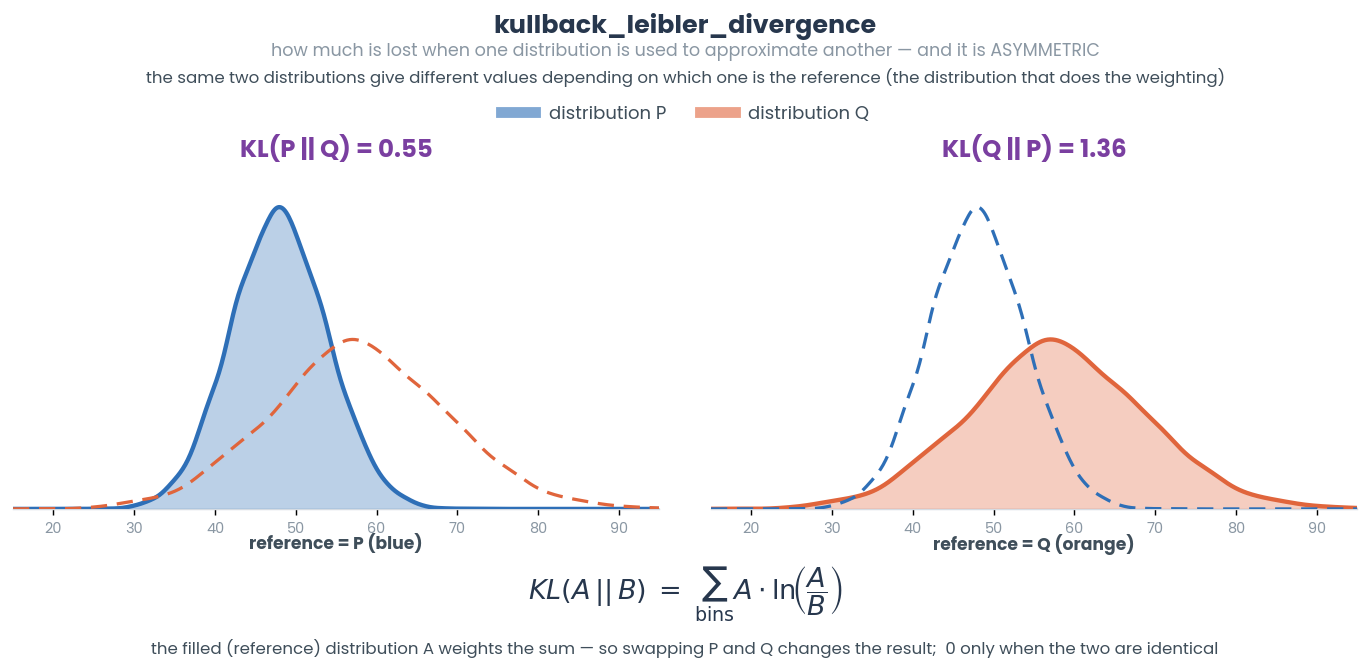

See also

For rolling comparisons in a timeseries, see simba.mixins.statistics_mixin.Statistics.rolling_kullback_leibler_divergence() For GPU implementation, see simba.data_processors.cuda.statistics.kullback_leibler_divergence_gpu().

Parameters

• sample_1 (ndarray) – First 1d array representing feature values.

• sample_2 (ndarray) – Second 1d array representing feature values.

• fill_value (Optional[int]) – Optional pseudo-value to use to fill empty buckets in sample_2 histogram

• bucket_method (Literal) – Estimator determining optimal bucket count and bucket width. Default: The maximum of the Sturges and Freedman-Diaconis estimators

Returns

Kullback-Leibler divergence between sample_1 and sample_2

Return type

float

kumar_hassebrook_similarity(x, y)

Kumar-Hassebrook similarity is a measure used to quantify the similarity between two vectors.

Note

Kumar-Hassebrook similarity score of 1 indicates identical vectors and 0 indicating no similarity

Parameters

• x (np.ndarray) – 1D array representing the first feature values.

• y (np.ndarray) – 1D array representing the second feature values.

Returns

Kumar-Hassebrook similarity between vectors x and y.

Return type

float

Example

>>> x, y = np.random.randint(0, 500, (1000,)), np.random.randint(0, 500, (1000,))
>>> Statistics.kumar_hassebrook_similarity(x=x, y=y)

static levenes(sample_1, sample_2, critical_values=None)

Compute Levene’s W statistic, a test for the equality of variances between two samples.

Levene’s test is a statistical test used to determine whether two or more groups have equal variances. It is often used as an alternative to the Bartlett test when the assumption of normality is violated. The function computes the Levene’s W statistic, which measures the degree of difference in variances between the two samples.

See also

For time-series based rolling comparisons, see simba.mixins.statistics_mixin.Statistics.rolling_levenes()

Parameters

• sample_1 (ndarray) – First 1d array representing feature values.

• sample_2 (ndarray) – Second 1d array representing feature values.

• critical_values (ndarray) – 2D array with where first column represent dfn first row dfd with values represent critical values. Can be found in simba.assets.critical_values_05.pickle

Returns

Levene’s W statistic and a boolean indicating whether the test is statistically significant (if critical values is not None).

Return type

Tuple[float, Union[bool, None]]

Examples

>>> sample_1 = np.array(list(range(0, 50)))
>>> sample_2 = np.array(list(range(25, 100)))
>>> Statistics().levenes(sample_1=sample_1, sample_2=sample_2)
>>> 12.63909108903254
>>> critical_values = pickle.load(open("simba/assets/lookups/critical_values_5.pickle","rb"))['f']['one_tail'].values
>>> Statistics().levenes(sample_1=sample_1, sample_2=sample_2, critical_values=critical_values)
>>> (12.63909108903254, True)

static local_outlier_factor(data, k=5, contamination=1e-10, normalize=False, groupby_idx=None)

Compute the local outlier factor of each observation.

Note

The final LOF scores are negated. Thus, higher values indicate more atypical (outlier) data points. Values Method calls sklearn.neighbors.LocalOutlierFactor directly. Attempted to use own jit compiled implementation, but runtime was 3x-ish slower than sklearn.neighbors.LocalOutlierFactor.

If groupby_idx is not None, then the index 1 of data array for which to group the data and compute LOF within each segment/cluster. E.g., can be field holding cluster identifier. Thus, outliers are computed within each segment/cluster, ensuring that other segments cannot affect outlier scores within each analyzing each cluster.

If groupby_idx is provided, then all observations with cluster/segment variable -1 will be treated as unclustered and assigned the max outlier score found withiin the clustered observations.

Parameters

• data (ndarray) – 2D array with feature values where rows represent frames and columns represent features.

• k (Union[int, float]) – Number of neighbors to evaluate for each observation. If the value is a float, then interpreted as the ratio of data.shape[0]. If the value is an integer, then it represent the number of neighbours to evaluate.

• contamination (Optional[float]) – Small pseudonumber to avoid DivisionByZero error.

• normalize (Optional[bool]) – Whether to normalize the distances between 0 and 1. Defaults to False.

• groupby_idx (Optional[int]) – If int, then the index 1 of data for which to group the data and compute LOF on each segment. E.g., can be field holding a cluster identifier.

Returns

Array of size data.shape[0] with local outlier scores.

Return type

np.ndarray

Example

>>> data, lbls = make_blobs(n_samples=2000, n_features=2, centers=10, random_state=42)
>>> data = np.hstack((data, lbls.reshape(-1, 1)))
>>> lof = Statistics.local_outlier_factor(data=data, groupby_idx=2, k=100, normalize=True)
>>> results = np.hstack((data[:, 0:2], lof.reshape(lof.shape[0], 1)))
>>> PlottingMixin.continuous_scatter(data=results, palette='seismic', bg_clr='lightgrey',size=30)

static mad_median_rule(data, k)

Detects outliers in the given data using the Median Absolute Deviation (MAD) rule. Returns a 1D array of size data.shape[0], where 1 represents an outlier and 0 represents an inlier.

See also

simba.mixins.timeseries_features_mixin.TimeseriesFeatureMixin.sliding_descriptive_statistics() simba.mixins.statistics_mixin.Statistics.sliding_mad_median_rule()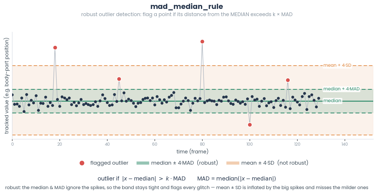

Parameters

• data (np.ndarray) – A 1-dimensional array of numerical values to check for outliers.

• k (int) – The multiplier for the MAD threshold. Higher values make the rule less sensitive to deviations from the median.

Returns

A 1D binary array of the same length as data, where each element is 1 if the corresponding element in data is classified as an outlier, and 0 otherwise.

Return type

np.ndarray

Example

>>> data = np.random.randint(0, 600, (9000000,)).astype(np.float32)
>>> Statistics.mad_median_rule(data=data, k=1)

static mahalanobis_distance_cdist(data)

Compute the Mahalanobis distance between every pair of observations in a 2D array using numba.

The Mahalanobis distance is a measure of the distance between a point and a distribution. It accounts for correlations between variables and the scales of the variables, making it suitable for datasets where features are not independent and have different variances.

Note

Significantly reduced runtime versus Mahalanobis scipy.cdist only with larger feature sets ( > 10-50).

However, Mahalanobis distance may not be suitable in certain scenarios, such as: - When the dataset is small and the covariance matrix is not accurately estimated. - When the dataset contains outliers that significantly affect the estimation of the covariance matrix. - When the assumptions of multivariate normality are violated.

Parameters

data (np.ndarray) – 2D array with feature observations. Frames on axis 0 and feature values on axis 1

Returns

Pairwise Mahalanobis distance matrix where element (i, j) represents the Mahalanobis distance between observations i and j.

Return type

np.ndarray

Example

>>> data = np.random.randint(0, 50, (1000, 200)).astype(np.float32)
>>> x = Statistics.mahalanobis_distance_cdist(data=data)

static manhattan_distance_cdist(data)

Compute the pairwise Manhattan distance matrix between points in a 2D array.

Can be preferred over Euclidean distance in scenarios where the movement is restricted to grid-based paths and/or the data is high dimensional.

\[D_{\text{Manhattan}} = |x_2 - x_1| + |y_2 - y_1|\]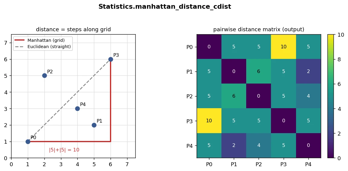

Parameters

data – 2D array where each row represents a featurized observation (e.g., frame)

Return np.ndarray

Pairwise Manhattan distance matrix where element (i, j) represents the distance between points i and j.

Example

>>> data = np.random.randint(0, 50, (10000, 2))
>>> Statistics.manhattan_distance_cdist(data=data)

static mann_whitney(sample_1, sample_2)

Jitted compute of Mann-Whitney U between two distributions.

The Mann-Whitney U test is used to assess whether the distributions of two groups are the same or different based on their ranks. It is commonly used as an alternative to the t-test when the assumptions of normality and equal variances are violated.

\[U = \min(U_1, U_2)\]

Where:

• \(U\) is the Mann-Whitney U statistic,

• \(U_1\) is the sum of ranks for sample 1,

• \(U_2\) is the sum of ranks for sample 2.

Parameters

• sample_1 (ndarray) – First 1d array representing feature values.

• sample_2 (ndarray) – Second 1d array representing feature values.

:return : The Mann-Whitney U statistic. :rtype: float

References

Modified from James Webber gist on GitHub.

Example

>>> sample_1 = np.array([1, 1, 3, 4, 5])
>>> sample_2 = np.array([6, 7, 8, 9, 10])
>>> results = Statistics().mann_whitney(sample_1=sample_1, sample_2=sample_2)

static mclain_rao_index(x, y)

Computes the McClain-Rao Index, which measures the quality of clustering by evaluating the ratio of the mean within-cluster distances to the mean between-cluster distances.

The McClain-Rao Index is computed by calculating the mean ratio of intra-cluster distances (distances between points within the same cluster) to inter-cluster distances (distances between points from different clusters). A lower value indicates a better clustering result, with clusters being compact and well-separated.

Parameters

• x (np.ndarray) – The dataset as a 2D NumPy array of shape (n_samples, n_features).

• y (np.ndarray) – Cluster labels for each data point as a 1D NumPy array of shape (n_samples,).

Returns

The McClain-Rao Index score, a lower value indicates better clustering quality.

Return type

float

References

1

McClain, J. O., & Rao, V. R. (1975). CLUSTISZ: A program to test for the quality of clustering of a set of objects. *Journal of Marketing Research, 12*(4), 456-460. https://doi.org/10.1177/002224377501200410

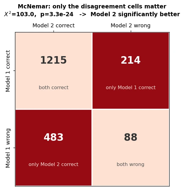
static mcnemar(x, y, ground_truth, continuity_corrected=True)

Perform McNemar’s test to compare the predictive accuracy of two models. This test is used to evaluate if the accuracies of two classifiers are significantly different when tested on the same data.

The chi-squared statistic (with continuity correction if continuity_corrected=True) is calculated as:

\[X^2 = \frac{(|b - c| - 1)^2}{b + c} \,\text{ if corrected, or }\, X^2 = \frac{(b - c)^2}{b + c}\]

where:

• b is the number of instances misclassified by the first model but correctly classified by the second model.

• c is the number of instances correctly classified by the first model but misclassified by the second model.

Note

Adapted from mlextend.

Parameters

• x (np.ndarray) – 1-dimensional Boolean array with predictions of the first model.

• y (np.ndarray) – 1-dimensional Boolean array with predictions of the second model.

• ground_truth (np.ndarray) – 1-dimensional Boolean array with ground truth labels.

• continuity_corrected (Optional[bool]) – Whether to apply continuity correction. Default is True.

Returns

McNemar score are significance level.

Return type

Tuple[float, float]

Example

>>> x = np.random.randint(0, 2, (100000, ))
>>> y = np.random.randint(0, 2, (100000, ))
>>> ground_truth = np.random.randint(0, 2, (100000, ))
>>> Statistics.mcnemar(x=x, y=y, ground_truth=ground_truth)

static normalized_google_distance(x, y)

Compute the Normalized Google Distance (NGD) between two vectors or matrices.

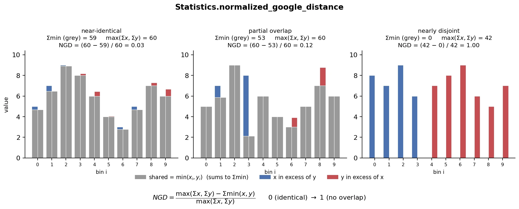
Normalized Google Distance is a measure of similarity between two sets based on the relationship between the sums and minimum values of their elements.

The NGD is calculated as:

\[NGD(x, y) = \frac{\max(\sum x, \sum y) - \sum \min(x, y)}{(\sum x + \sum y) - \min(\sum x, \sum y)}\]

where: - \(\sum x\) is the sum of elements in x - \(\sum y\) is the sum of elements in y - \(\sum \min(x, y)\) is the sum of element-wise minimums of x and y

Note

This function assumes x and y have the same shape. It computes NGD based on the sum of elements and the minimum values between corresponding elements of x and y.

Parameters

• x (np.ndarray) – First numerical matrix with shape (m, n).

• y (np.ndarray) – Second array or matrix with shape (m, n).

Returns

Normalized Google Distance between x and y.

Return type

float

Example

>>> x, y = np.random.randint(0, 500, (1000,200)), np.random.randint(0, 500, (1000,200))
>>> Statistics.normalized_google_distance(x=y, y=x)

References

1

Cilibrasi, R., & Vitányi, P. (2007). Clustering by compression. IEEE Transactions on Information Theory, 51(4), 1523-1545. https://doi.org/10.1109/TIT.2005.862080

static one_way_anova(sample_1, sample_2, critical_values=None)

Compute the one-way ANOVA F-statistic and associated p-value for two distributions.

This method calculates the F-statistic to determine if there is a significant difference between the means of the two samples, based on their variances. The F-statistic is computed as:

\[F = \frac{MS_{\text{between}}}{MS_{\text{within}}}\]

where: - \(SS_{\text{between}}\) is the sum of squares between the groups. - \(SS_{\text{within}}\) is the sum of squares within each group. - \(MS_{\text{between}} = \frac{SS_{\text{between}}}{df_{\text{between}}}\) - \(MS_{\text{within}} = \frac{SS_{\text{within}}}{df_{\text{within}}}\)

See also

For rolling comparisons in a timeseries, see simba.mixins.statistics_mixin.Statistics.rolling_one_way_anova()

Parameters

• sample_1 (np.ndarray) – First 1d array representing feature values.

• sample_2 (np.ndarray) – Second 1d array representing feature values.

Returns

Tuple representing ANOVA F statistic and associated probability value.

Return type

Tuple[float, float]

Example

>>> sample_1 = np.array([1, 2, 3, 1, 3, 2, 1, 10, 8, 4, 10])
>>> sample_2 = np.array([8, 5, 5, 8, 8, 9, 10, 1, 7, 10, 10])
>>> Statistics().one_way_anova(sample_1=sample_2, sample_2=sample_1)

static one_way_anova_scipy(x, y, variable_names, x_name='', y_name='')

Compute one-way ANOVAs comparing each column (axis 1) on two arrays.

Note

Use for computing and presenting aggregate statistics. Not suitable for featurization.

See also

For featurization instead use simba.mixins.statistics_mixin.Statistics.rolling_one_way_anova() or simba.mixins.statistics_mixin.Statistics.one_way_anova()

Parameters

• x (np.ndarray) – First 2d array with observations rowwise and variables columnwise.

• y (np.ndarray) – Second 2d array with observations rowwise and variables columnwise. Must be same number of columns as x.

• variable_names (List[str, ...]) – Names of columnwise variable names. Same length as number of data columns.

• x_name (str) – Name of the first group (x).

• y_name (str) – Name of the second group (y).

Returns

Dataframe with one row per column representing the ANOVA F-statistic and P-values comparing the variables between x and y.

Return type

pd.DataFrame

static pairwise_tukeyhsd_scipy(data, group, variable_names, verbose=False)

Compute pairwise grouped Tukey-HSD tests.

Note

Use for computing and presenting aggregate statistics. Not suitable for featurization.

Parameters

• data (np.ndarray) – 2D array with observations rowwise (axis 0) and features columnwise (axis 1)

• group (np.ndarray) – 1D array with the same number of observations as rows in data containing the group for each sample.

• variable_names (List[str, ...]) – Names of columnwise variable names. Same length as number of data columns.

Returns

Dataframe comparing each group for each variable.

Return type

pd.DataFrame

static pbm_index(x, y)

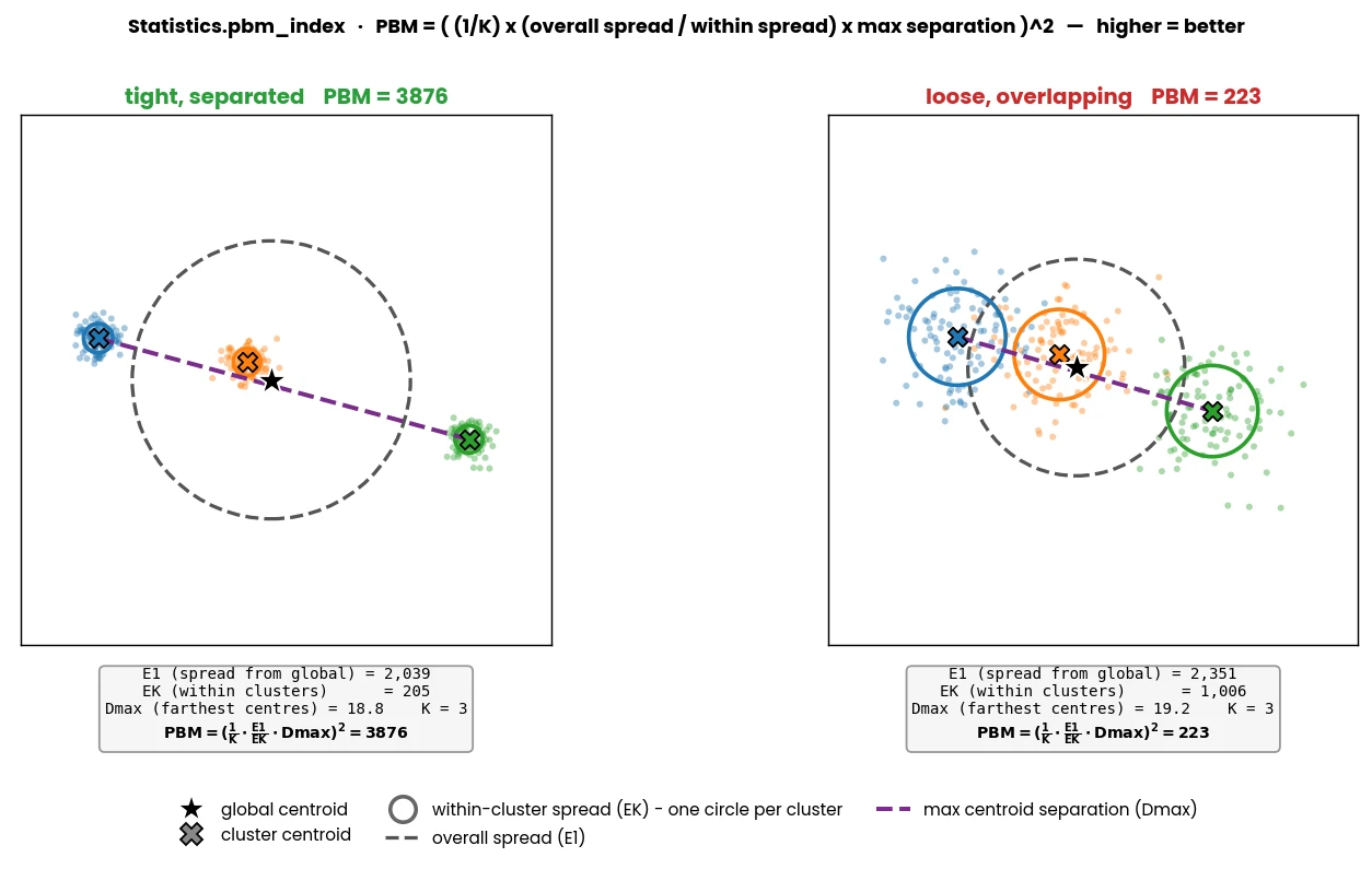
Compute the PBM (Performance of the Best Matching) Index, a measure of clustering quality that combines the compactness of the clusters and the separation between them. The PBM index evaluates how well-defined the clusters are in terms of their intra-cluster distance and the distance between their centroids.

Higher values indicates better clustering.

Parameters

• x (np.ndarray) – A 2D array of shape (n_samples, n_features) containing the data points.

• y (np.ndarray) – A 1D array of shape (n_samples,) containing cluster labels for the data points.

Returns

The PBM Index value.

Return type

float

References

1

Pakhira, M. K., Bandyopadhyay, S., & Maulik, U. (2004). Validity index for crisp and fuzzy clusters. Pattern Recognition, 37(3), 487–501.

2

Desgraupes, B. clusterCrit: Clustering Indices (R package vignette). CRAN.

Example

>>> X, y = make_blobs(n_samples=5, centers=2, n_features=3, random_state=0, cluster_std=5)
>>> Statistics.pbm_index(x=X, y=y)

static pct_in_top_n(x, n)

Compute the percentage of elements in the top ‘n’ frequencies in the input array.

This function calculates the percentage of elements that belong to the ‘n’ most frequent categories in the input array ‘x’.

Parameters

• x (np.ndarray) – Input array.

• n (float) – Number of top frequencies.

Returns

Percentage of elements in the top ‘n’ frequencies.

Return type

float

Example

>>> x = np.random.randint(0, 10, (100,))
>>> Statistics.pct_in_top_n(x=x, n=5)

static pearsons_r(sample_1, sample_2)

Calculate the Pearson correlation coefficient (Pearson’s r) between two numeric samples.

Pearson’s r is a measure of the linear correlation between two sets of data points. It quantifies the strength and direction of the linear relationship between the two variables. The coefficient varies between -1 and 1, with -1 indicating a perfect negative linear relationship, 1 indicating a perfect positive linear relationship, and 0 indicating no linear relationship.

Pearson’s r is calculated using the formula:

\[r = \frac{\sum{(x_i - \bar{x})(y_i - \bar{y})}}{\sqrt{\sum{(x_i - \bar{x})^2}\sum{(y_i - \bar{y})^2}}}\]

where:

• \(x_i\) and \(y_i\) are individual data points in sample_1 and sample_2, respectively.

• \(\bar{x}\) and \(\bar{y}\) are the means of sample_1 and sample_2, respectively.

See also

For timeseries-based sliding comparison, see simba.mixins.statistics_mixin.Statistics.sliding_pearsons_r()

Parameters

• sample_1 (np.ndarray) – First numeric sample.

• sample_2 (np.ndarray) – Second numeric sample.

Returns

Pearson’s correlation coefficient between the two samples.

Return type

float

Example

>>> sample_1 = np.array([7, 2, 9, 4, 5, 6, 7, 8, 9]).astype(np.float32)
>>> sample_2 = np.array([1.5, 2.5, 3.5, 4.5, 5.5, 6.5, 7.5, 8.5, 9.5]).astype(np.float32)
>>> Statistics().pearsons_r(sample_1=sample_1, sample_2=sample_2)
>>> 0.47

static phi_coefficient(data)

Compute the phi coefficient for a Nx2 array of binary data.

The phi coefficient (a.k.a Matthews Correlation Coefficient (MCC)), is a measure of association for binary data in a 2x2 contingency table. It quantifies the degree of association or correlation between two binary variables (e.g., binary classification targets).

The formula for the phi coefficient is defined as:

\[\phi = \frac{{(BC - AD)}}{{\sqrt{{(C\_1 + C\_2)(R\_1 + R\_2)(C\_1 + R\_1)(C\_2 + R\_2)}}}}\]

where:

• \(BC\): Hit rate (reponse and truth is both 1)

• \(AD\): Correct rejections (response and truth are both 0)

• \(C1, C2\): Counts of occurrences where the response is 1 and 0, respectively.

• math`R1, R2`

  Counts of occurrences where the truth is 1 and 0, respectively.

See also

For time-series based sliding comparisons, see simba.mixins.statistics_mixin.Statistics.sliding_phi_coefficient()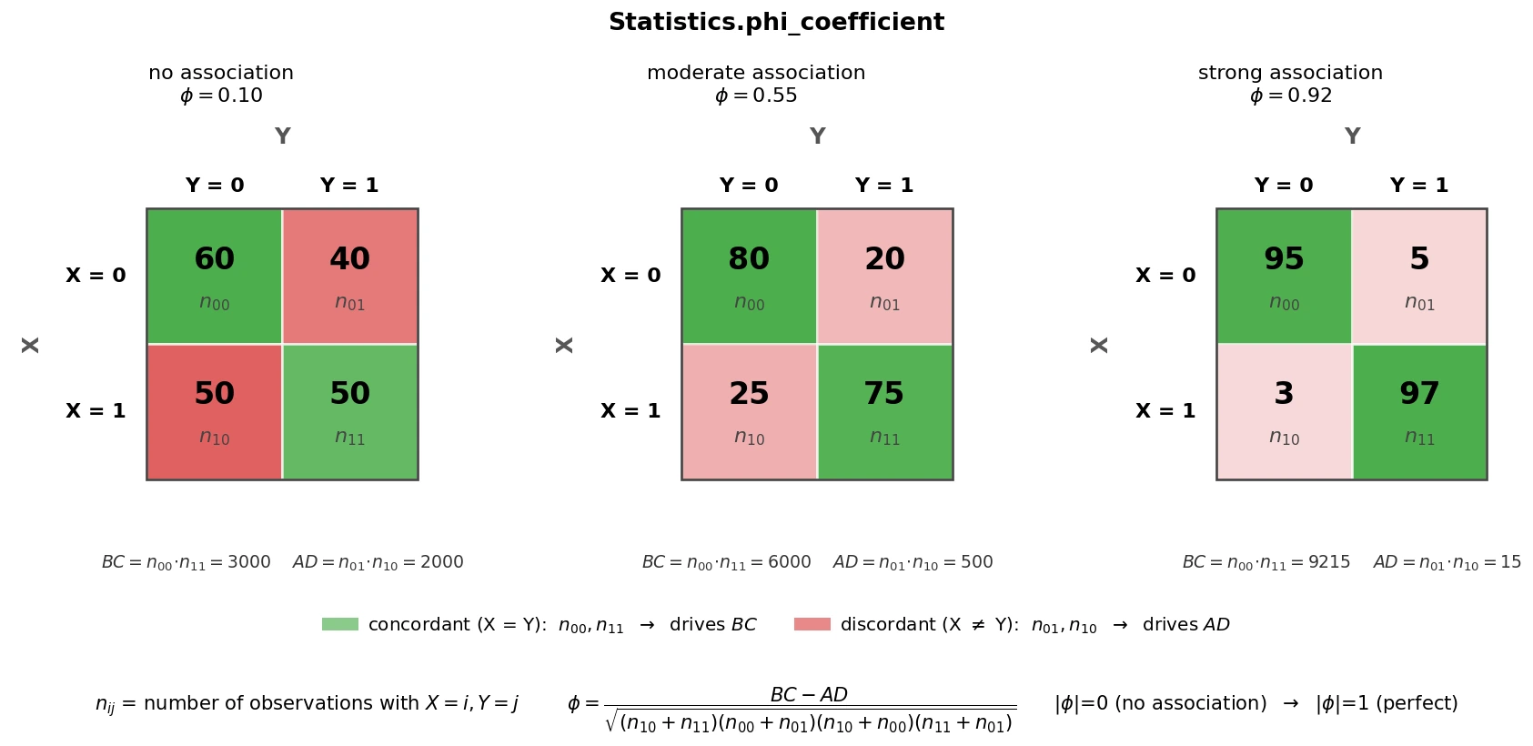

Parameters

data (np.ndarray) – A NumPy array containing binary data organized in two columns. Each row represents a pair of binary values for two variables. Columns represent two features or two binary classification results.

Returns

The calculated phi coefficient, a value between 0 and 1. A value of 0 indicates no association between the variables, while 1 indicates a perfect association.

Return type

float

Example

>>> data = np.array([[0, 1], [1, 0], [1, 0], [1, 1]]).astype(np.int64)
>>> Statistics().phi_coefficient(data=data)
>>> 0.5773502691896258
>>> data = np.random.randint(0, 2, (100, 2))
>>> result = Statistics.phi_coefficient(data=data)

population_stability_index(sample_1, sample_2, fill_value=1, bucket_method='auto')

Compute Population Stability Index (PSI) comparing two distributions.

The Population Stability Index (PSI) is a measure of the difference in distribution patterns between two groups of data. A low PSI value indicates a minimal or negligible change in the distribution patterns between the two samples. A high PSI value suggests a significant difference in the distribution patterns between the two samples.

Note

Empty bins (0 observations in bin) in is replaced with fill_value. The PSI value ranges from 0 to positive infinity.

The Population Stability Index (PSI) is calculated as:

\[PSI = \sum \left(p_2 - p_1\right) \cdot \ln\left(\frac{{p_2}}{{p_1}}\right)\]

where:

• \(p_1\) and \(p_2\) are the proportions of observations in the bins for sample 1 and sample 2 respectively.

See also

For time-series based rolling comparisons, see simba.mixins.statistics_mixin.Statistics.rolling_population_stability_index()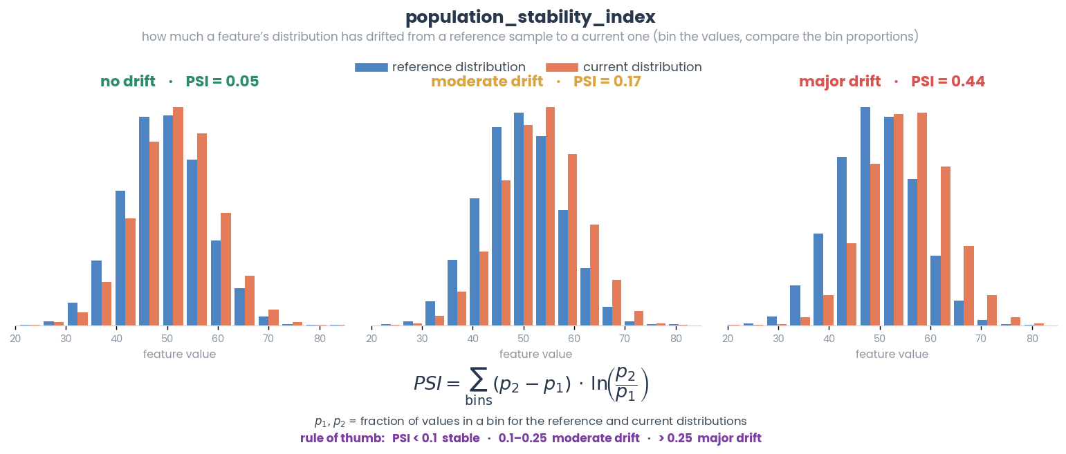

Parameters

• sample_1 (ndarray) – First 1d array representing feature values.

• sample_2 (ndarray) – Second 1d array representing feature values.

• fill_value (Optional[int]) – Empty bins (0 observations in bin) in is replaced with fill_value. Default 1.

• bucket_method (Literal) – Estimator determining optimal bucket count and bucket width. Default: The maximum of the Sturges and Freedman-Diaconis estimators

Returns

PSI distance between sample_1 and sample_2

Return type

float

Example

>>> sample_1, sample_2 = np.random.randint(0, 100, (100,)), np.random.randint(0, 10, (100,))
>>> Statistics().population_stability_index(sample_1=sample_1, sample_2=sample_2, fill_value=1, bucket_method='auto')
>>> 3.9657026867553817

static ray_turi_index(x, y)

Compute the Ray-Turi index for evaluating the clustering quality.

A lower value indicates a better clustering result.

Parameters

• x (np.ndarray) – The dataset as a 2D NumPy array of shape (n_samples, n_features).

• y (np.ndarray) – Cluster labels for each data point as a 1D NumPy array of shape (n_samples,).

Returns

The Ray-Turi index score.

Return type

float

Example

>>> from sklearn.datasets import make_blobs
>>> X, labels = make_blobs(n_samples=5000, centers=5, random_state=42, n_features=3, cluster_std=2)
>>> score = Statistics.s_dbw_index(X, labels)

References

1

Ray, S., & Turi, R. H. (1999). Determination of number of clusters in k-means clustering and application in colour image segmentation. Proceedings of the 4th International Conference on Advances in Pattern Recognition and Digital Techniques, 137–143.

static relative_risk(x, y)

Calculate the relative risk between two binary arrays.

Relative risk (RR) is the ratio of the probability of an event occurring in one group/feature/cluster/variable (x) to the probability of the event occurring in another group/feature/cluster/variable (y).

See also

For time-series based sliding data, use simba.mixins.statistics_mixin.Statistics.sliding_relative_risk()

Parameters

• x (np.ndarray) – The first 1D binary array.

• y (np.ndarray) – The second 1D binary array.

Returns

The relative risk between arrays x and y.

Return type

float

Example

>>> Statistics.relative_risk(x=np.array([0, 1, 1]), y=np.array([0, 1, 0]))
>>> 2.0

static rmsstd(x, y)

Compute the Root-Mean-Square Standard Deviation (RMSSTD) for a clustering result.

Parameters

• x (np.ndarray) – A 2D array of shape (n_samples, n_features) representing the feature vectors of the data points.

• y (np.ndarray) – A 1D array of shape (n_samples,) containing the cluster labels for each data point.

Returns

The RMSSTD index value. Lower values indicate better clustering.

Return type

float

References

1

Milligan, G. W., & Cooper, M. C. (1985). An examination of procedures for determining the number of clusters in a data set. Psychometrika, 50(2), 159–179.

Example

>>> X, y = make_blobs(n_samples=100, centers=10, n_features=3, random_state=0, cluster_std=0.1)
>>> d = Statistics.rmsstd(x=X, y=y)

static rolling_barletts_test(data, time_windows, fps)

Compute rolling Bartlett’s test statistic comparing variances between consecutive time windows.

Bartlett’s test is used to test the null hypothesis that the variances of two or more groups are equal. This function splits the data into consecutive time windows and compares the variance of each window to the variance of the preceding window. The test statistic follows a chi-square distribution under the null hypothesis of equal variances.

Note

The first time window (where there is no preceding window) will have fill value 0.0. The test assumes that the data within each window is approximately normally distributed.

The Bartlett’s test statistic (\(u\)) is calculated as:

\[u = \frac{(N - 2) \cdot (\ln(\sigma_1^2) + \ln(\sigma_2^2))}{\frac{1}{n_1 - 1} + \frac{1}{n_2 - 1}}\]

where:

• \(N = n_1 + n_2\) is the total number of observations

• \(n_1\) and \(n_2\) are the sample sizes of the two consecutive windows

• \(\sigma_1^2\) and \(\sigma_2^2\) are the sample variances of the two windows

See also

For Levene’s test (more robust to non-normality), see simba.mixins.statistics_mixin.Statistics.rolling_levenes().

Parameters

• data (np.ndarray) – 1D array of feature values to test.

• time_windows (np.ndarray) – Array of time window sizes in seconds. E.g., np.array([1.0, 2.0]) for 1s and 2s windows.

• fps (float) – Frames per second of the recorded video.

Returns

2D array of size len(data) x len(time_windows) containing Bartlett’s test statistics. Contains 0.0 for the first window of each time window size.

Return type

np.ndarray

Example

>>> data = np.random.normal(loc=0, scale=1, size=(100,)).astype(np.float32)
>>> Statistics().rolling_barletts_test(data=data, time_windows=np.array([1.0, 2.0]), fps=10.0)

static rolling_cohens_d(data, time_windows, fps)

Jitted compute of rolling Cohen’s D statistic comparing the current time-window of size N to the preceding window of size N.

See also

For single non-timeseries comparison, see simba.mixins.statistics_mixin.Statistics.cohens_d()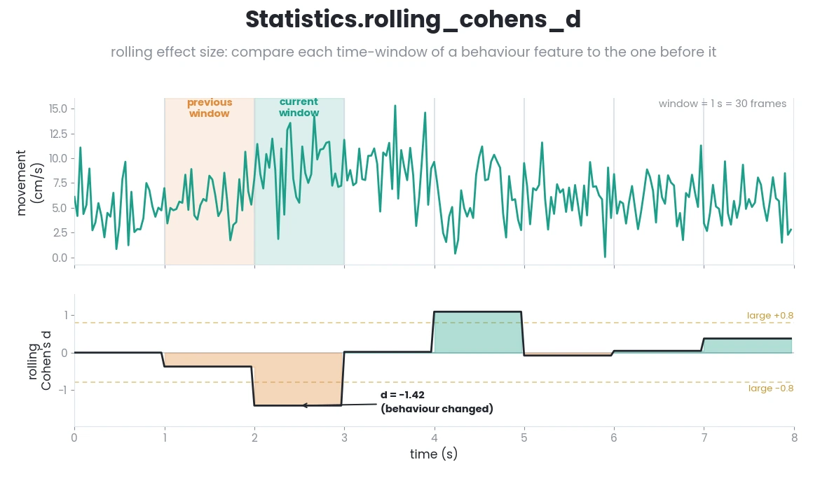

Parameters

• data (ndarray) – 1D array of size len(frames) representing feature values.

• time_window (np.ndarray[ints]) – Time windows to compute ANOVAs for in seconds.

• fps (int) – Frame-rate of recorded video.

Returns

Array of size data.shape[0] x window_sizes.shape[1] with Cohens D.

Return type

np.ndarray

Example

>>> sample_1, sample_2 = np.random.normal(loc=10, scale=1, size=4), np.random.normal(loc=11, scale=2, size=4)
>>> sample = np.hstack((sample_1, sample_2))
>>> Statistics().rolling_cohens_d(data=sample, window_sizes=np.array([1]), fps=4)
>>> [[0.],[0.],[0.],[0.],[0.14718302],[0.14718302],[0.14718302],[0.14718302]])

static rolling_independent_sample_t(data, time_window, fps)

Jitted compute independent-sample t-statistics for sequentially binned values in a time-series. E.g., compute t-test statistics when comparing Feature N in the current 1s time-window, versus Feature N in the previous 1s time-window.

Parameters

• data (ndarray) – 1D array of size len(frames) representing feature values.

• group_size_s (int) – The size of the buckets in seconds.

• fps – Frame-rate of recorded video.

Return type

int

Attention

Each window is compared to the prior window. Output for the windows without a prior window (the first window) is -1.

See also

For single non-timeseries independent t, see simba.mixins.statistics_mixin.Statistics.independent_samples_t()

Example

>>> data_1, data_2 = np.random.normal(loc=10, scale=2, size=10), np.random.normal(loc=20, scale=2, size=10)
>>> data = np.hstack([data_1, data_2])
>>> Statistics().rolling_independent_sample_t(data, time_window=1, fps=10)
>>> [[-1, -1, -1, -1, -1, -1, -1, -1, -1, -1, -6.88741389, -6.88741389, -6.88741389, -6.88741389, -6.88741389, -6.88741389, -6.88741389, -6.88741389, -6.88741389, -6.88741389])

rolling_jensen_shannon_divergence(data, time_windows, fps, bucket_method='auto')

Compute rolling Jensen-Shannon divergence comparing the current time-window of size N to the preceding window of size N.

See also

For simple two distribution comparison, see simba.mixins.statistics_mixin.Statistics.jensen_shannon_divergence()

Parameters

• data (ndarray) – 1D array of size len(frames) representing feature values.

• time_windows (np.ndarray[ints]) – Time windows to compute JS for in seconds.

• fps (int) – Frame-rate of recorded video.

• bucket_method (Literal) – Estimator determining optimal bucket count and bucket width. Default: The maximum of the Sturges and Freedman-Diaconis estimators

Returns

Array of size data.shape[0] x window_sizes.shape[0] with Jensen-Shannon divergence. Columns represents different time windows.

Return type

np.ndarray

rolling_kullback_leibler_divergence(data, time_windows, fps, fill_value=1, bucket_method='auto')

Compute rolling Kullback-Leibler divergence comparing the current time-window of size N to the preceding window of size N.

Note

Empty bins (0 observations in bin) in is replaced with fill_value.

See also

For single comparison between two distributions, see simba.mixins.statistics_mixin.Statistics.kullback_leibler_divergence()

Parameters

• sample_1 (ndarray) – 1d array representing feature values.

• bucket_method (Literal) – Estimator determining optimal bucket count and bucket width. Default: The maximum of the Sturges and Freedman-Diaconis estimators

• time_windows (np.ndarray[floats]) – Time windows to compute JS for in seconds.

• fps (int) – Frame-rate of recorded video.

Returns

Size data.shape[0] x window_sizes.shape with Kullback-Leibler divergence. Columns represents different tiem windows.

Return type

np.ndarray

Example

>>> sample_1, sample_2 = np.random.normal(loc=10, scale=700, size=5), np.random.normal(loc=50, scale=700, size=5)
>>> data = np.hstack((sample_1, sample_2))
>>> Statistics().rolling_kullback_leibler_divergence(data=data, time_windows=np.array([1]), fps=2)

static rolling_levenes(data, time_windows, fps)

Jitted compute of rolling Levene’s W comparing the current time-window of size N to the preceding window of size N.

Note

First time bin (where has no preceding time bin) will have fill value 0

See also

For simple two-sample comparison, see simba.mixins.statistics_mixin.Statistics.levenes()

Parameters

• sample_1 (ndarray) – First 1d array representing feature values.

• sample_2 (ndarray) – Second 1d array representing feature values.

Returns

Levene’s W data of size len(data) x len(time_windows).

Return type

np.ndarray

Example

>>> data = np.random.randint(0, 50, (100)).astype(np.float64)
>>> Statistics().rolling_levenes(data=data, time_windows=np.array([1]).astype(np.float64), fps=5.0)

static rolling_mann_whitney(data, time_windows, fps)

Jitted compute of rolling Mann-Whitney U comparing the current time-window of size N to the preceding window of size N.

Note

First time bin (where has no preceding time bin) will have fill value 0

Modified from James Webber gist.

See also

For simple two-distribution comparion, see simba.mixins.statistics_mixin.Statistics.mann_whitney().

Parameters

• sample_1 (ndarray) – First 1d array representing feature values.

• sample_2 (ndarray) – Second 1d array representing feature values.

Returns

Mann-Whitney U data of size len(data) x len(time_windows).

Return type

np.ndarray

Examples

>>> data = np.random.randint(0, 4, (200)).astype(np.float32)
>>> results = Statistics().rolling_mann_whitney(data=data, time_windows=np.array([1.0]), fps=1)

static rolling_one_way_anova(data, time_windows, fps)

Jitted compute of rolling one-way ANOVA F-statistic comparing the current time-window of size N to the preceding window of size N.

See also

For single comparison, see simba.mixins.statistics_mixin.Statistics.one_way_anova()

Parameters

• data (ndarray) – 1D array of size len(frames) representing feature values.

• time_windows (np.ndarray[ints]) – Time windows to compute ANOVAs for in seconds.

• fps (int) – Frame-rate of recorded video.

Returns

2D numpy array with F values comparing the current time-window to the immedidatly preceeding time-window.

Return type

np.ndarray

Example

>>> sample = np.random.normal(loc=10, scale=1, size=10).astype(np.float32)
>>> Statistics().rolling_one_way_anova(data=sample, time_windows=np.array([1.0]), fps=2)
>>> [[0.00000000e+00][0.00000000e+00][2.26221263e-06][2.26221263e-06][5.39119950e-03][5.39119950e-03][1.46725486e-03][1.46725486e-03][1.16392111e-02][1.16392111e-02]]

rolling_population_stability_index(data, time_windows, fps, fill_value=1, bucket_method='auto')

Compute rolling Population Stability Index (PSI) comparing the current time-window of size N to the preceding window of size N.

Note

Empty bins (0 observations in bin) in is replaced with fill_value.

See also

For simple two-distribution comparisons, see simba.mixins.statistics_mixin.Statistics.population_stability_index().

Parameters

• sample_1 (ndarray) – First 1d array representing feature values.

• sample_2 (ndarray) – Second 1d array representing feature values.

• fill_value (int) – Empty bins (0 observations in bin) in is replaced with fill_value.

• bucket_method (Literal) – Estimator determining optimal bucket count and bucket width. Default: The maximum of the Sturges and Freedman-Diaconis estimators

Returns

PSI data of size len(data) x len(time_windows).

Return type

np.ndarray

rolling_shapiro_wilks(data, time_window, fps)

Compute Shapiro-Wilks normality statistics for sequentially binned values in a time-series. E.g., compute the normality statistics of Feature N in each window of time_window seconds.

Parameters

• data (ndarray) – 1D array of size len(frames) representing feature values.

• time_window (int) – The size of the buckets in seconds.

• fps (int) – Frame-rate of recorded video.

Returns

Array of size data.shape[0] with Shapiro-Wilks normality statistics

Return type

np.ndarray

Example

>>> data = np.random.randint(low=0, high=100, size=(200)).astype('float32')
>>> results = self.rolling_shapiro_wilks(data=data, time_window=1, fps=30)

static rolling_two_sample_ks(data, time_window, fps)

Jitted compute Kolmogorov two-sample statistics for sequentially binned values in a time-series. E.g., compute KS statistics when comparing Feature N in the current 1s time-window, versus Feature N in the previous 1s time-window.

See also

For single non-timeseries based comparison, see simba.mixins.statistics_mixin.Statistics.two_sample_ks()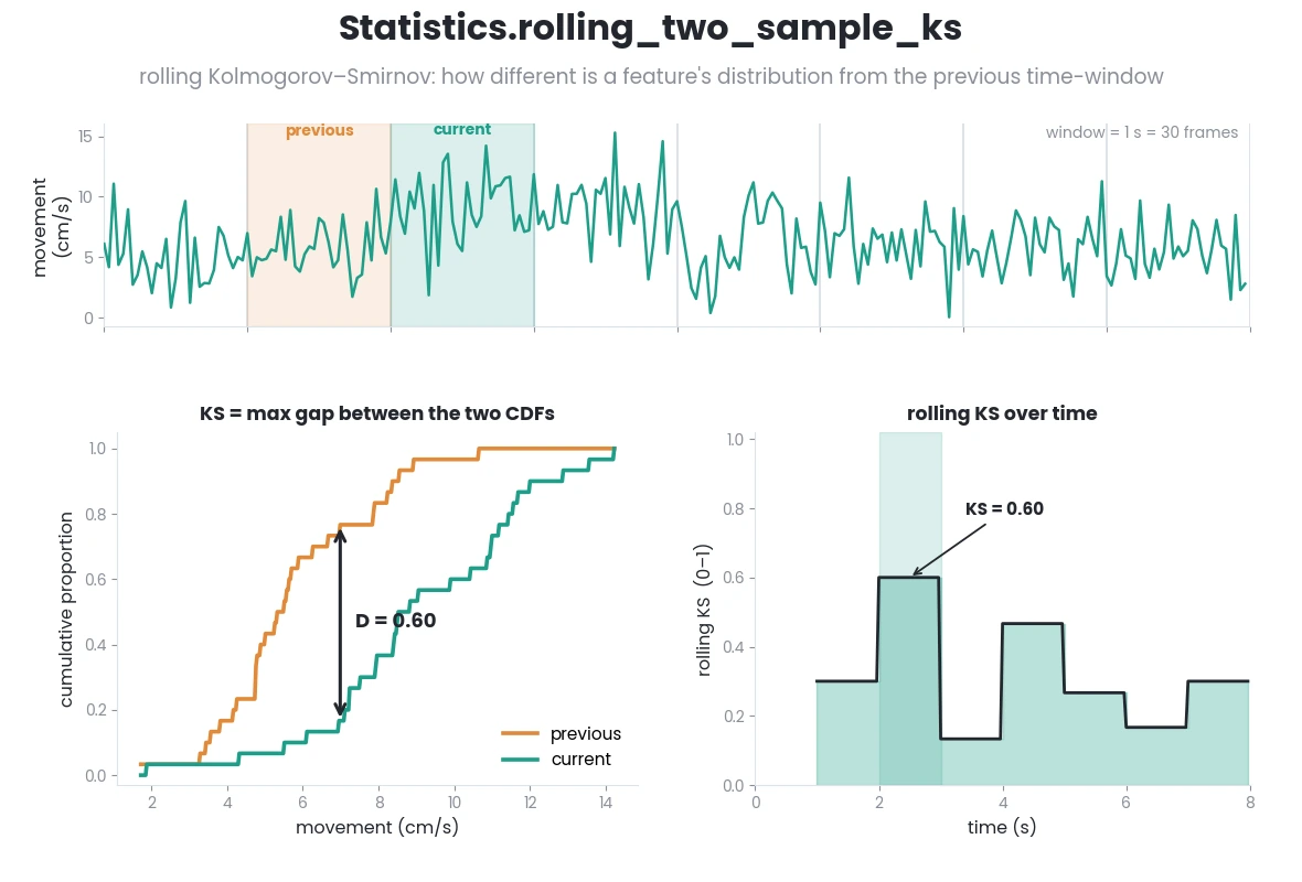

Parameters

• data (ndarray) – 1D array of size len(frames) representing feature values.

• time_window (float) – The size of the buckets in seconds.

• fps (int) – Frame-rate of recorded video.

Returns

Array of size data.shape[0] with KS statistics

Return type

np.ndarray

Example

>>> data = np.random.randint(low=0, high=100, size=(200)).astype('float32')
>>> results = Statistics().rolling_two_sample_ks(data=data, time_window=1, fps=30)

rolling_wasserstein_distance(data, time_windows, fps, bucket_method='auto')

Compute rolling Wasserstein distance comparing the current time-window of size N to the preceding window of size N.

See also

For simple two distribution earth mover comparison, see simba.mixins.statistics_mixin.Statistics.wasserstein_distance()

Parameters

• data (ndarray) – 1D array of size len(frames) representing feature values.

• time_windows (np.ndarray[ints]) – Time windows to compute JS for in seconds.

• fps (int) – Frame-rate of recorded video.

• bucket_method (Literal) – Estimator determining optimal bucket count and bucket width. Default: The maximum of the Sturges and Freedman-Diaconis estimators

Returns

Size data.shape[0] x window_sizes.shape with Wasserstein distance. Columns represent different time windows.

Return type

np.ndarray

Example

>>> data = np.random.randint(0, 100, (100,))
>>> Statistics().rolling_wasserstein_distance(data=data, time_windows=np.array([1, 2]), fps=30)

static s_dbw_index(x, y)

Compute the S_Dbw index for evaluating the clustering quality.

A lower value indicates a better clustering result.

Parameters

• x (np.ndarray) – The dataset as a 2D NumPy array of shape (n_samples, n_features).

• y (np.ndarray) – Cluster labels for each data point as a 1D NumPy array of shape (n_samples,).

Returns

The S_Dbw index score.

Return type

float

Note

Behaves weird as the number of dimensions increase (> 20).

Example

>>> from sklearn.datasets import make_blobs
>>> X, labels = make_blobs(n_samples=5000, centers=5, random_state=42, n_features=3, cluster_std=2)
>>> score = Statistics.s_dbw_index(X, labels)

References

1

Halkidi, M., & Vazirgiannis, M. (2001). Clustering validity assessment: finding the optimal partitioning of a data set. Proceedings IEEE International Conference on Data Mining, 187–194.

static scott_symons_index(x, y)

Compute the Scott-Symons index for clustering evaluation.

Smaller values represent better clustering. Values can be negative.

Parameters

• x (np.ndarray) – The dataset as a 2D NumPy array of shape (n_samples, n_features).

• y (np.ndarray) – Cluster labels for each data point as a 1D NumPy array of shape (n_samples,).

Returns

The Scott-Symons index score.

Return type

float

References

1

Scott, A. J., & Symons, M. J. (1971). Clustering methods based on likelihood ratio criteria. Biometrics, 27(2), 387–397.

static sd_index(x, y)

Compute the SD (Scatter and Discriminant) Index for evaluating the quality of a clustering solution.

The SD Index combines two components to measure clustering quality: 1. Scatter (SCAT): Evaluates the compactness of clusters by measuring the ratio of intra-cluster variance to the global standard deviation. 2. Discriminant (DIS): Measures the separation between clusters relative to their distance from the global mean.

A lower SD Index indicates better clustering quality, reflecting compact and well-separated clusters.

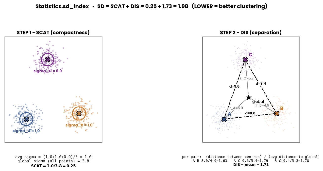
Parameters

• x (np.ndarray) – A 2D array of shape (n_samples, n_features) representing the feature vectors of the data points.

• y (np.ndarray) – A 1D array of shape (n_samples,) containing the cluster labels for each data point.

Returns

The SD Index value. Lower values indicate better clustering quality with more compact and well-separated clusters.

Return type

float

Example

>>> X, y = make_blobs(n_samples=800, centers=2, n_features=3, random_state=0, cluster_std=0.1)
>>> Statistics.sd_index(x=X, y=y)

References

1

Halkidi, M., Vazirgiannis, M., & Batistakis, Y. (2000). Quality scheme assessment in the clustering process (PKDD 2000). Principles of Data Mining and Knowledge Discovery, Lecture Notes in Computer Science, vol. 1910. Springer.

silhouette_score(x, y)

Compute the silhouette score for the given dataset and labels.

See also

For GPU implementation, see simba.data_processors.cuda.statistics.silhouette_score_gpu()

Parameters

• x (np.ndarray) – The dataset as a 2D NumPy array of shape (n_samples, n_features).

• y (np.ndarray) – Cluster labels for each data point as a 1D NumPy array of shape (n_samples,).

Returns

The average silhouette score for the dataset.

Return type

float

Example

>>> x, y = make_blobs(n_samples=10000, n_features=400, centers=5, cluster_std=10, center_box=(-1, 1))
>>> score = silhouette_score(x=x, y=y)

>>> from sklearn.metrics import silhouette_score as sklearn_silhouette # SKLEARN ALTERNATIVE
>>> score_sklearn = sklearn_silhouette(x, y)

static sliding_autocorrelation(data, max_lag, time_window, fps)

Jitted computation of sliding autocorrelations, which measures the correlation of a feature with itself using lagged windows.

Parameters

• data (np.ndarray) – 1D array containing feature values.

• max_lag (float) – Maximum lag in seconds for the autocorrelation window.

• time_window (float) – Length of the sliding time window in seconds.

• fps (float) – Frames per second, used to convert time-related parameters into frames.

Returns

1D array containing the sliding autocorrelation values.

Return type

np.ndarray

Example

>>> data = np.array([0,1,2,3,4, 5,6,7,8,1,10,11,12,13,14]).astype(np.float32)
>>> Statistics().sliding_autocorrelation(data=data, max_lag=0.5, time_window=1.0, fps=10)
>>> [ 0., 0., 0.,  0.,  0., 0., 0.,  0. ,  0., -3.686, -2.029, -1.323, -1.753, -3.807, -4.634]

static sliding_cumulative_mean(x)

Compute a sliding cumulative mean over a 1D

Parameters

x (np.ndarray) – A 1D NumPy array of type float32

Returns

A 1D float32 array of the same shape as x, containing the cumulative mean at each index, ignoring NaNs.

Return type

np.ndarray

static sliding_czebyshev_distance(x, window_sizes, sample_rate)

Calculate the sliding Chebyshev distance for a given signal with different window sizes.

This function computes the sliding Chebyshev distance for a signal x using different window sizes specified by window_sizes. The Chebyshev distance measures the maximum absolute difference between the corresponding elements of two signals.

Note

Normalize array x before passing it to ensure accurate results.

See also

For simple 2-sample comparison, use simba.mixins.statistics_mixin.Statistics.czebyshev_distance()

Parameters

• x (np.ndarray) – Input signal, a 2D array with shape (n_samples, n_features).

• window_sizes (np.ndarray) – Array containing window sizes for sliding computation.

• sample_rate (float) – Sampling rate of the signal.

Returns

2D array of Chebyshev distances for each window size and position.

Return type

np.ndarray

Example

>>> sample_1 = np.random.randint(0, 10, (200,5)).astype(np.float32)
>>> sample_2 = np.random.randint(0, 10, (10000,100))
>>> Statistics.sliding_czebyshev_distance(x=sample_1, window_sizes=np.array([1.0, 2.0]), sample_rate=10.0)

static sliding_dominant_frequencies(data, fps, k, time_windows, window_function=None)

Find the K dominant frequencies within a feature vector using sliding windows

static sliding_eta_squared(x, y, window_sizes, sample_rate)

Calculate sliding window eta-squared, a measure of effect size for between-subjects designs, over multiple window sizes.

See also

For two-sample comparison, see simba.mixins.statistics_mixin.Statistics.eta_squared()

Parameters

• x (np.ndarray) – The array containing the dependent variable data.

• y (np.ndarray) – The array containing the grouping variable (categorical) data.

• window_sizes (np.ndarray) – 1D array of window sizes in seconds.

• sample_rate (int) – The sampling rate of the data in frames per second.

Returns

Array of size x.shape[0] x window_sizes.shape[0] with sliding eta squared values.

Return type

np.ndarray

Example

>>> x = np.random.randint(0, 10, (10000,))
>>> y = np.random.randint(0, 2, (10000,))
>>> Statistics.sliding_eta_squared(x=x, y=y, window_sizes=np.array([1.0, 2.0]), sample_rate=10)

static sliding_independent_samples_t(data, time_window, slide_time, critical_values, fps)

Jitted compute of sliding independent sample t-test. Compares the feature values in current time-window to prior time-windows to find the length in time to the most recent time-window where a significantly different feature value distribution is detected.

See also

For simple two distribution commparison, see simba.mixins.statistics_mixin.Statistics.independent_samples_t()

Parameters

• data (ndarray) – 1D array with feature values.

• time_window (float) – The sizes of the two feature value windows being compared in seconds.

• slide_time (float) – The slide size of the second window.

• critical_values (ndarray) – 2D array with where indexes represent degrees of freedom and values represent critical T values. Can be found in simba.assets.critical_values_05.pickle.

• fps (int) – The fps of the recorded video.

Returns

1D array of size len(data) with values representing time to most recent significantly different feature distribution.

Return type

np.ndarray

Example

>>> data = np.random.randint(0, 50, (10)).astype(np.float32)
>>> critical_values = pickle.load(open("simba/assets/lookups/critical_values_05.pickle", "rb"))['independent_t_test']['one_tail'].values.astype(np.float32)
>>> results = Statistics().sliding_independent_samples_t(data=data, time_window=0.5, fps=5.0, critical_values=critical_values, slide_time=0.30)

static sliding_iqr(x, window_size, sample_rate)

Compute the sliding interquartile range (IQR) for a 1D array of feature values.

Parameters

• x (ndarray) – 1D array representing the feature values for which the IQR will be calculated.

• window_size (float) – Size of the sliding window, in seconds. This value determines how many samples are included in each window.

• sample_rate (float) – The sampling rate in samples per second, e.g., fps.

:return : Sliding IQR values :rtype: np.ndarray

References

1

Hession, Leinani E., Gautam S. Sabnis, Gary A. Churchill, and Vivek Kumar. “A Machine-Vision-Based Frailty Index for Mice.” Nature Aging 2, no. 8 (August 16, 2022): 756–66. https://doi.org/10.1038/s43587-022-00266-0.

Example

>>> data = np.random.randint(0, 50, (90,)).astype(np.float32)
>>> window_size = 0.5
>>> Statistics.sliding_iqr(x=data, window_size=0.5, sample_rate=10.0)

static sliding_kendall_tau(sample_1, sample_2, time_windows, fps)

Compute sliding Kendall’s Tau correlation coefficient.

Calculates Kendall’s Tau correlation coefficient between two samples over sliding time windows. Kendall’s Tau is a measure of correlation between two ranked datasets.

The computation is based on the formula:

\[\tau = \frac{{\text{{concordant pairs}} - \text{{discordant pairs}}}}{{\text{{concordant pairs}} + \text{{discordant pairs}}}}\]

where concordant pairs are pairs of elements with the same order in both samples, and discordant pairs are pairs with different orders.

See also

For simple two-sample comparison, see simba.mixins.statistics_mixin.Statistics.kendall_tau().

References

1

Stephanie Glen, “Kendall’s Tau (Kendall Rank Correlation Coefficient)”.

Parameters

• sample_1 (np.ndarray) – First sample for comparison.

• sample_2 (np.ndarray) – Second sample for comparison.

• time_windows (np.ndarray) – Rolling time windows in seconds.

• fps (float) – Frames per second (FPS) of the recorded video.

Returns

Array of Kendall’s Tau correlation coefficients corresponding to each time window.

Return type

np.ndarray

static sliding_kurtosis(data, time_windows, sample_rate)

Compute the kurtosis of a 1D array within sliding time windows.

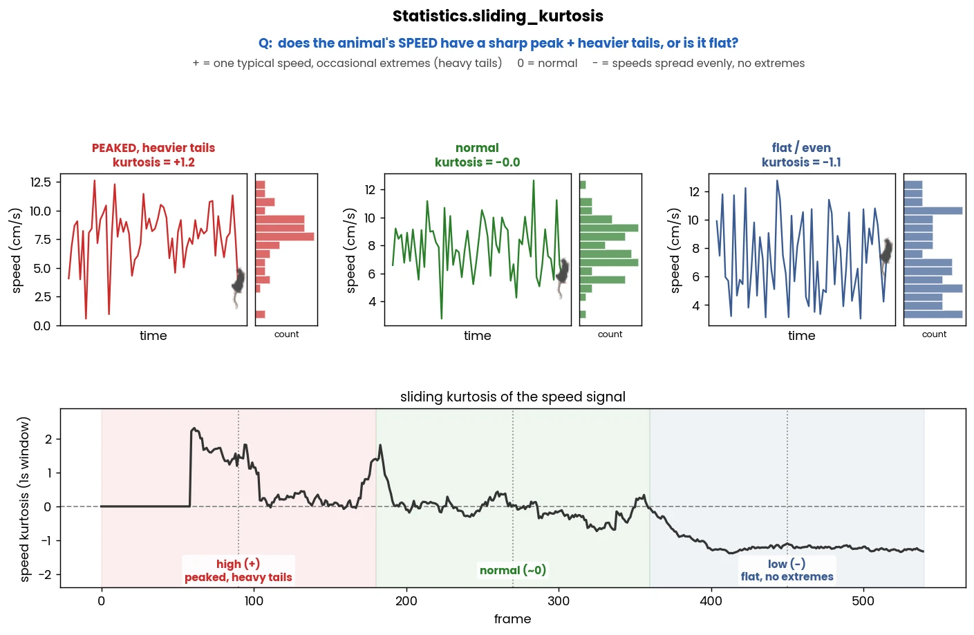
Parameters

• data (np.ndarray) – Input data array.

• time_windows (np.ndarray) – 1D array of time window durations in seconds.

• sample_rate (np.ndarray) – Sampling rate of the data in samples per second.

Return np.ndarray

2D array of skewness`1 values with rows corresponding to data points and columns corresponding to time windows.

Example

>>> data = np.random.randint(0, 100, (10,))
>>> kurtosis = Statistics().sliding_kurtosis(data=data.astype(np.float32), time_windows=np.array([1.0, 2.0]), sample_rate=2)

static sliding_mad_median_rule(data, k, time_windows, fps)

Count the number of outliers in a sliding time-window using the MAD-Median Rule.

The MAD-Median Rule is a robust method for outlier detection. It calculates the median absolute deviation (MAD) and uses it to identify outliers based on a threshold defined as k times the MAD.

See also

For alternative method, see simba.mixins.timeseries_features_mixin.TimeseriesFeatureMixin.sliding_descriptive_statistics() For single dataset, use simba.mixins.statistics_mixin.Statistics.mad_median_rule()

Parameters

• data (np.ndarray) – 1D numerical array representing feature.

• k (int) – The outlier threshold defined as k * median absolute deviation in each time window.

• time_windows (np.ndarray) – 1D array of time window sizes in seconds.

• fps (float) – The frequency of the signal.

Returns

Array of size (data.shape[0], time_windows.shape[0]) with counts if outliers detected.

Return type

np.ndarray

Example

>>> data = np.random.randint(0, 50, (50000,)).astype(np.float32)
>>> Statistics.sliding_mad_median_rule(data=data, k=2, time_windows=np.array([20.0]), fps=1.0)

static sliding_pearsons_r(sample_1, sample_2, time_windows, fps)

Given two 1D arrays of size N, create sliding window of size time_windows[i] * fps and return Pearson’s R between the values in the two 1D arrays in each window. Address “what is the correlation between Feature 1 and Feature 2 in the current X.X seconds of the video”.

See also

For simple two sample comparison, see simba.mixins.statistics_mixin.Statistics.pearsons_r()

Parameters

• sample_1 (ndarray) – First 1D array with feature values.

• sample_2 (ndarray) – Second 1D array with feature values.

• time_windows (float) – The length of the sliding window in seconds.

• fps (int) – The fps of the recorded video.

Returns

2d array of Pearsons R of size len(sample_1) x len(time_windows). Note, if sliding window is 10 frames, the first 9 entries will be filled with 0.

Return type

np.ndarray

Example

>>> sample_1 = np.random.randint(0, 50, (10)).astype(np.float32)
>>> sample_2 = np.random.randint(0, 50, (10)).astype(np.float32)
>>> Statistics().sliding_pearsons_r(sample_1=sample_1, sample_2=sample_2, time_windows=np.array([0.5]), fps=10)
>>> [[-1.][-1.][-1.][-1.][0.227][-0.319][-0.196][0.474][-0.061][0.713]]

static sliding_phi_coefficient(data, window_sizes, sample_rate)

Calculate sliding phi coefficients for a 2x2 contingency table derived from binary data.

Computes sliding phi coefficients for a 2x2 contingency table derived from binary data over different time windows. The phi coefficient is a measure of association between two binary variables, and sliding phi coefficients can reveal changes in association over time.

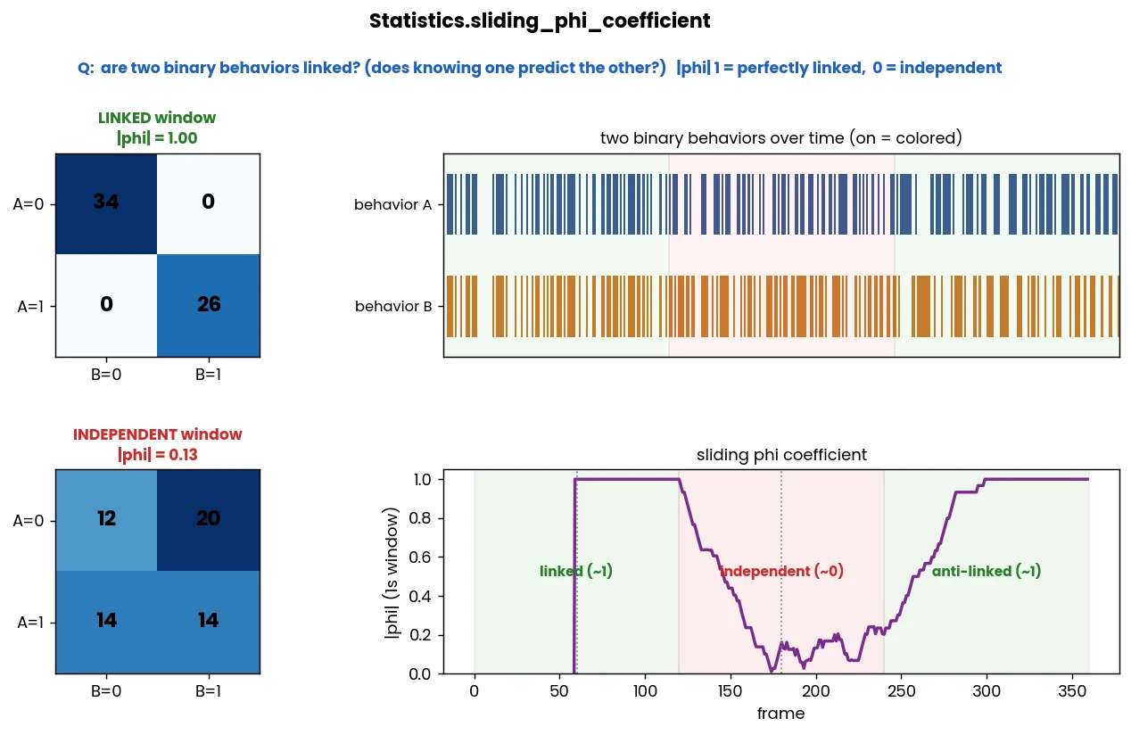
See also

For simple two distribution comparison, see simba.mixins.statistics_mixin.Statistics.phi_coefficient().

Parameters

• data (np.ndarray) – A 2D NumPy array containing binary data organized in two columns. Each row represents a pair of binary values for two variables.

• window_sizes (np.ndarray) – 1D NumPy array specifying the time windows (in seconds) over which to calculate the sliding phi coefficients.

• sample_rate (int) – The sampling rate or time interval (in samples per second, e.g., fps) at which data points were collected.

Returns

A 2D NumPy array containing the calculated sliding phi coefficients. Each row corresponds to the phi coefficients calculated for a specific time point, the columns correspond to time-windows.

Return type

np.ndarray

Example

>>> data = np.random.randint(0, 2, (200, 2))
>>> Statistics().sliding_phi_coefficient(data=data, window_sizes=np.array([1.0, 4.0]), sample_rate=10)

static sliding_relative_risk(x, y, window_sizes, sample_rate)

Calculate sliding relative risk values between two binary arrays using different window sizes.

See also

For single two distribution comparion, use simba.mixins.statistics_mixin.Statistics.relative_risk()

Parameters

• x (np.ndarray) – The first 1D binary array.

• y (np.ndarray) – The second 1D binary array.

• window_sizes (np.ndarray) – One-dimensional array with the time-windows in seconds.

• sample_rate (int) – The sample rate of the input data (e.g., FPS).

Return np.ndarray

Array of size x.shape[0] x window_sizes.shape[0] with sliding eta squared values.

Example

>>> Statistics.sliding_relative_risk(x=np.array([0, 1, 1, 0]), y=np.array([0, 1, 0, 0]), window_sizes=np.array([1.0]), sample_rate=2)

static sliding_skew(data, time_windows, sample_rate)

Compute the skewness of a 1D array within sliding time windows.

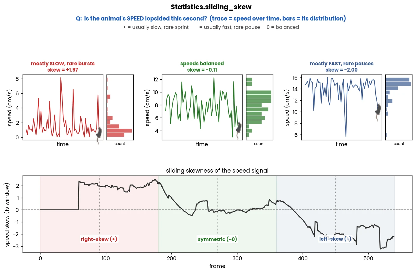
Parameters

• data (np.ndarray) – 1D array of input data.

• time_windows (np.ndarray) – 1D array of time window durations in seconds.

• sample_rate (np.ndarray) – Sampling rate of the data in samples per second.

Return np.ndarray

2D array of skewness`1 values with rows corresponding to data points and columns corresponding to time windows.

Example

>>> data = np.random.randint(0, 100, (10,))
>>> skewness = Statistics().sliding_skew(data=data.astype(np.float32), time_windows=np.array([1.0, 2.0]), sample_rate=2)

static sliding_spearman_rank_correlation(sample_1, sample_2, time_windows, fps)

Given two 1D arrays of size N, create sliding window of size time_windows[i] * fps and return Spearman’s rank correlation between the values in the two 1D arrays in each window. Address “what is the correlation between Feature 1 and Feature 2 in the current X.X seconds of the video.

See also

For simple two-distribution comparion, see simba.mixins.statistics_mixin.Statistics.spearman_rank_correlation().

Parameters

• sample_1 (ndarray) – First 1D array with feature values.

• sample_2 (ndarray) – Second 1D array with feature values.

• time_windows (float) – The length of the sliding window in seconds.

• fps (int) – The fps of the recorded video.

Returns

2d array of Soearman’s ranks of size len(sample_1) x len(time_windows). Note, if sliding window is 10 frames, the first 9 entries will be filled with 0. The 10th value represents the correlation in the first 10 frames.

Return type

np.ndarray

Example

>>> sample_1 = np.array([9,10,13,22,15,18,15,19,32,11]).astype(np.float32)
>>> sample_2 = np.array([11, 12, 15, 19, 21, 26, 19, 20, 22, 19]).astype(np.float32)
>>> Statistics().sliding_spearman_rank_correlation(sample_1=sample_1, sample_2=sample_2, time_windows=np.array([0.5]), fps=10)

static sliding_z_scores(data, time_windows, fps)

Calculate sliding Z-scores for a given data array over specified time windows.

This function computes sliding Z-scores for a 1D data array over different time windows. The sliding Z-score is a measure of how many standard deviations a data point is from the mean of the surrounding data within the specified time window. This can be useful for detecting anomalies or variations in time-series data.

Parameters

• data (ndarray) – 1D NumPy array containing the time-series data.

• time_windows (ndarray) – 1D NumPy array specifying the time windows in seconds over which to calculate the Z-scores.

• fps (int) – Frames per second, used to convert time windows from seconds to the corresponding number of data points.

Returns

A 2D NumPy array containing the calculated Z-scores. Each row corresponds to the Z-scores calculated for a specific time window. The time windows are represented by the columns.

Return type

np.ndarray

Example

>>> data = np.random.randint(0, 100, (1000,)).astype(np.float32)
>>> z_scores = Statistics().sliding_z_scores(data=data, time_windows=np.array([1.0, 2.5]), fps=10)

static sokal_michener(x, y, w=None)

Jitted compute of the Sokal-Michener dissimilarity between two binary vectors or matrices.

Higher values indicate more dissimilar vectors or matrices, while lower values indicate more similar vectors or matrices.

The Sokal-Michener dissimilarity is a measure of dissimilarity between two sets based on the presence or absence of similar attributes. This implementation supports weighted dissimilarity.

Note

Adapted from umap.

\[D(x, y) = \frac{2 \cdot \sum_{i} w_i \cdot \mathbb{1}(x_i \neq y_i)}{N + \sum_{i} w_i \cdot \mathbb{1}(x_i \neq y_i)}\]

where: - \(x\) and \(y\) are the binary vectors or matrices. - \(w_i\) is the weight for the i-th element. - \(\mathbb{1}(x_i \neq y_i)\) is an indicator function that is 1 if \(x_i \neq y_i\) and 0 otherwise. - \(N\) is the total number of elements in \(x\) or \(y\).

Parameters

• x (np.ndarray) – First binary vector or matrix.

• y (np.ndarray) – Second binary vector or matrix.

• w (Optional[np.ndarray]) – Optional weight vector. If None, all weights are considered as 1.

Returns

Sokal-Michener dissimilarity between x and y.

Return type

float

Example

>>> x = np.random.randint(0, 2, (200,))
>>> y = np.random.randint(0, 2, (200,))
>>> sokal_michener = Statistics.sokal_michener(x=x, y=y)

static sokal_sneath(x, y, w=None)

Jitted calculate of the sokal sneath coefficient between two binary vectors (e.g., to classified behaviors). 0 represent independence, 1 represents complete interdependence.

\[Sokal-Sneath = \frac{{f_t + t_f}}{{2 \cdot (t_{{cnt}} + f_{{cnt}}) + f_t + t_f}}\]

Note

Adapted from pynndescent.

See also

For GPU method, see simba.data_processors.cuda.statistics.sokal_sneath_gpu()

Parameters

• x (np.ndarray) – First binary vector.

• y (np.ndarray) – Second binary vector.

• w (Optional[np.ndarray]) – Optional weights for each element. Can be classification probabilities. If not provided, equal weights are assumed.

Returns

sokal sneath coefficient

Return type

float

Example

>>> x = np.array([0, 1, 0, 0, 1]).astype(np.int8)
>>> y = np.array([1, 0, 1, 1, 0]).astype(np.int8)
>>> Statistics().sokal_sneath(x, y)
>>> 0.0

static spearman_rank_correlation(sample_1, sample_2)

Jitted compute of Spearman’s rank correlation coefficient between two samples.

Spearman’s rank correlation coefficient assesses how well the relationship between two variables can be described using a monotonic function. It computes the strength and direction of the monotonic relationship between ranked variables.

See also

For time-series based sliding comparisons, see simba.mixins.statistics.StatisticsMixin.sliding_spearman_rank_correlation() For time-series based sliding comparisons with GPU acceleration, see simba.data_processors.cuda.statistics.sliding_spearman_rank_correlation(),

Parameters

• sample_1 (np.ndarray) – First 1D array containing feature values.

• sample_2 (np.ndarray) – Second 1D array containing feature values.

Returns

Spearman’s rank correlation coefficient.

Return type

float

Example

>>> sample_1 = np.array([7, 2, 9, 4, 5, 6, 7, 8, 9]).astype(np.float32)
>>> sample_2 = np.array([1.5, 2.5, 3.5, 4.5, 5.5, 6.5, 7.5, 8.5, 9.5]).astype(np.float32)
>>> Statistics().spearman_rank_correlation(sample_1=sample_1, sample_2=sample_2)
>>> 0.0003979206085205078

static symmetry_index(x, y, agg_type='mean')

Calculate the Symmetry Index (SI) between two arrays of measurements, x and y, over a given time series. The Symmetry Index quantifies the relative difference between two measurements at each time point, expressed as a percentage. The function returns either the mean or median Symmetry Index over the entire series, based on the specified aggregation type.

Zero indicates perfect symmetry. Positive values represent increasing asymmetry between the two measurements.

The Symmetry Index (SI) is calculated as:

\[SI = \frac{|x_i - y_i|}{0.5 \times (x_i + y_i)} \times 100\]

where \(x_i\) and \(y_i\) are the values of the two measurements at each time point.

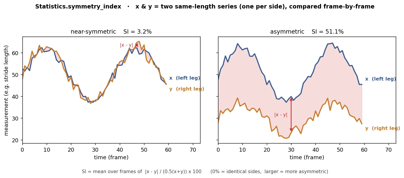
Parameters

• x (np.ndarray) – A 1-dimensional array of measurements from one side (e.g., left side), representing a time series or sequence of measurements.

• y (np.ndarray) – A 1-dimensional array of measurements from the other side (e.g., right side), of the same length as x.

• agg_type (Literal['mean', 'median']) – The aggregation method used to summarize the Symmetry Index across all time points.

Returns

The aggregated Symmetry Index over the series, either as the mean or median SI.

Return type

float

Example

>>> x = np.random.randint(0, 155, (100,))
>>>y = np.random.randint(0, 155, (100,))
>>> Statistics.symmetry_index(x=x, y=y)

static total_variation_distance(x, y, bucket_method='auto')

Calculate the total variation distance between two probability distributions.

Parameters

• x (np.ndarray) – A 1-D array representing the first sample.

• y (np.ndarray) – A 1-D array representing the second sample.

• bucket_method (Optional[str]) – The method used to determine the number of bins for histogram computation. Supported methods are ‘fd’ (Freedman-Diaconis), ‘doane’, ‘auto’, ‘scott’, ‘stone’, ‘rice’, ‘sturges’, and ‘sqrt’. Defaults to ‘auto’.

Returns

The total variation distance between the two distributions.

Return type

float

\[TV(P, Q) = 0.5 \sum_i |P_i - Q_i|\]

where \(P_i\) and \(Q_i\) are the probabilities assigned by the distributions \(P\) and \(Q\) to the same event \(i\), respectively.

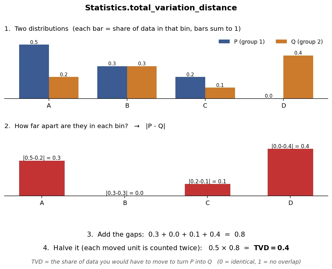
Example

>>> total_variation_distance(x=np.array([1, 5, 10, 20, 50]), y=np.array([1, 5, 10, 100, 110]))
>>> 0.3999999761581421

static two_sample_ks(sample_1, sample_2, critical_values=None)

Jitted compute the two-sample Kolmogorov-Smirnov (KS) test statistic and, optionally, test for statistical significance.

The two-sample KS test is a non-parametric test that compares the cumulative distribution functions (ECDFs) of two independent samples to assess whether they come from the same distribution.

KS statistic (D) is calculated as the maximum absolute difference between the empirical cumulative distribution functions (ECDFs) of the two samples.

\[D = \max(| ECDF_1(x) - ECDF_2(x) |)\]

If critical_values are provided, the function checks the significance of the KS statistic against the critical values.

See also

For rolling timeseries based comparison, see simba.mixins.statistics_mixin.Statistics.rolling_two_sample_ks()

Parameters

• sample_1 (np.ndarray) – The first sample array for the KS test.

• sample_2 (np.ndarray) – The second sample array for the KS test.

• critical_values (Optional[float64[:, :]]) – An array of critical values for the KS test. If provided, the function will also check the significance of the KS statistic against the critical values. Default: None.

Return (float Union[bool, None])

Returns a tuple containing the KS statistic and a boolean indicating whether the test is statistically significant.

Example

>>> sample_1 = np.array([1, 2, 3, 1, 3, 2, 1, 10, 8, 4, 10]).astype(np.float32)
>>> sample_2 = np.array([10, 5, 10, 4, 8, 10, 7, 10, 7, 10, 10]).astype(np.float32)
>>> critical_values = pickle.load(open("simba/assets/lookups/critical_values_5.pickle", "rb"))['two_sample_KS']['one_tail'].values
>>> Statistics.two_sample_ks(sample_1=sample_1, sample_2=sample_2, critical_values=critical_values)
>>> (0.6363636363636364, True)

wasserstein_distance(sample_1, sample_2, bucket_method='auto')

Compute Wasserstein distance between two distributions.

Note

Uses stats.wasserstein_distance. I have tried to move stats.wasserstein_distance to jitted method extensively, but this doesn’t give significant runtime improvement. Rate-limiter appears to be the _hist_1d.

See also

For time-series based comparisons, see simba.mixins.statistics_mixin.Statistics.rolling_wasserstein_distance()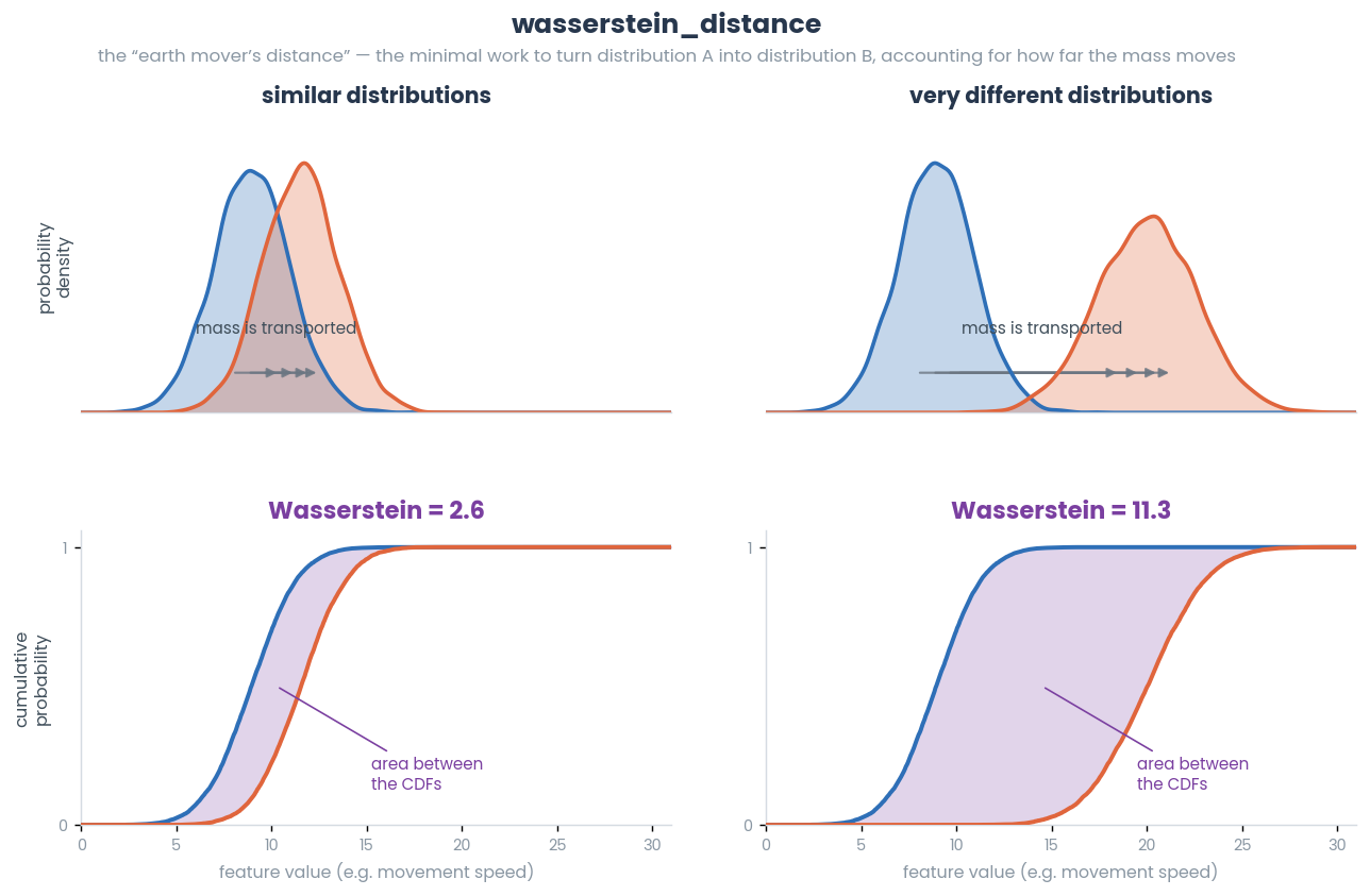

Parameters

• sample_1 (ndarray) – First 1d array representing feature values.

• sample_2 (ndarray) – Second 1d array representing feature values.

• bucket_method (Literal) – Estimator determining optimal bucket count and bucket width. Default: The maximum of the Sturges and Freedman-Diaconis estimators

Returns

Wasserstein distance between sample_1 and sample_2

Return type

float

Example

>>> sample_1 = np.random.normal(loc=10, scale=2, size=10000)
>>> sample_2 = np.random.normal(loc=12, scale=2, size=10000)
>>> Statistics().wasserstein_distance(sample_1=sample_1, sample_2=sample_2)
>>> 2.0  # ~ the 2-unit shift between the distributions

wave_hedges_distance(x, y)

Computes the Wave-Hedges distance between two 1-dimensional arrays x and y. The Wave-Hedges distance is a measure of dissimilarity between arrays.

Note

Wave-Hedges distance score of 0 indicate identical arrays. There is no upper bound.

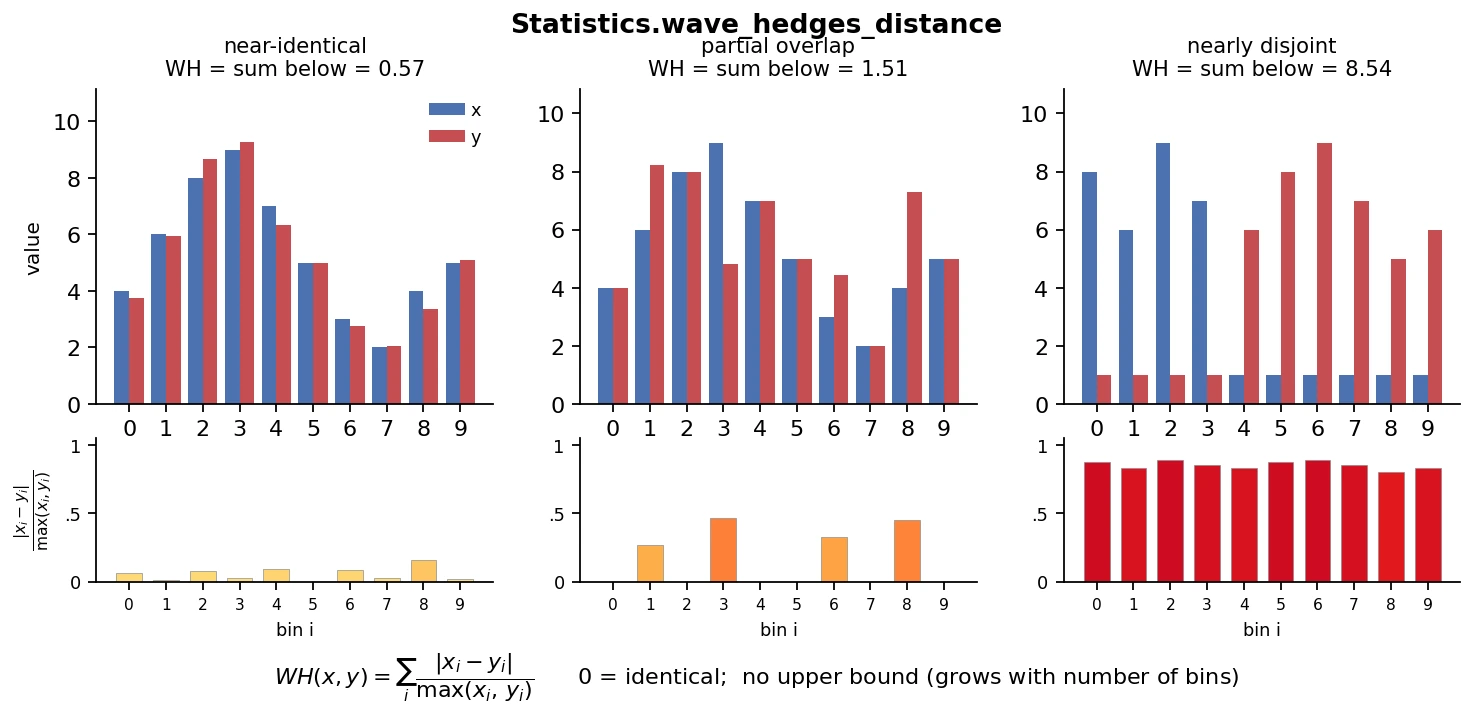
Parameters

• x (np.ndarray) – 1D array representing the first feature values.

• y (np.ndarray) – 1D array representing the second feature values.

Returns

Wave-Hedges distance

Return type

float

Example

>>> x = np.random.randint(0, 500, (1000,))
>>> y = np.random.randint(0, 500, (1000,))
>>> Statistics().wave_hedges_distance(x=x, y=y)

References

1

Hedges, T. S. (1976). An empirical modification to linear wave theory. Proceedings of the Institution of Civil Engineers, Part 2, 61(3), 575–579. https://doi.org/10.1680/iicep.1976.3408

static wemmert_gancarski_index(x, y)

Compute the Wemmert-Gançarski index for clustering evaluation.

The best case is when the index approaches 1, indicating good clustering. The worst case is when the index approaches 0, indicating poor clustering.

Parameters

• x (np.ndarray) – The dataset as a 2D NumPy array of shape (n_samples, n_features).

• y (np.ndarray) – Cluster labels for each data point as a 1D NumPy array of shape (n_samples,).

Returns

The Wemmert-Gançarski index score.

Return type

float

References

1

Bernard Desgraupes, University Paris Ouest Lab Modal’X, https://cran.r-project.org/web/packages/clusterCrit/vignettes/clusterCrit.pdf

static wilcoxon(x, y)

Perform the Wilcoxon signed-rank test for paired samples.

Wilcoxon signed-rank test is a non-parametric statistical hypothesis test used to compare two related samples, matched samples, or repeated measurements on a single sample to assess whether their population mean ranks differ.

Parameters

• x (np.ndarray) – 1D array representing the observations for the first sample.

• y (np.ndarray) – 1D array representing the observations for the second sample.

Returns

A tuple containing the test statistic (z-score) and the effect size (r).

• The test statistic (z-score) measures the deviation of the observed ranks sum from the expected sum.

• The effect size (r) measures the strength of association between the variables.

Return type

Tuple[float, float]

static xie_beni(x, y)

Computes the Xie-Beni index for clustering evaluation.

The score is calculated as the ratio between the average intra-cluster variance and the squared minimum distance between cluster centroids. This ensures that the index penalizes both loosely packed clusters and clusters that are too close to each other.

A lower Xie-Beni index indicates better clustering quality, signifying well-separated and compact clusters.

See also

To compute Xie-Beni on the GPU, use xie_beni(). Significant GPU savings detected at about 1m features, 25 clusters

\[\text{XB} = \frac{\frac{1}{n} \sum_{i=1}^{n} \| x_i - c_{y_i} \|^2}{\min_{i \neq j} \| c_i - c_j \|^2}\]

where \(n\) is the total number of points in the dataset, \(x_i\) is the \(i\)-th data point, \(c_{y_i}\) is the centroid of the cluster to which \(x_i\) belongs, and \(\| \cdot \|\) denotes the Euclidean norm.

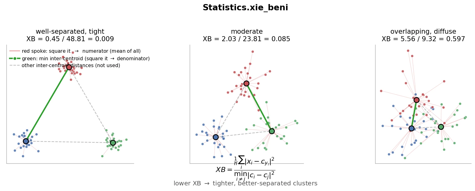
Parameters

• x (np.ndarray) – The dataset as a 2D NumPy array of shape (n_samples, n_features).

• y (np.ndarray) – Cluster labels for each data point as a 1D NumPy array of shape (n_samples,).

Returns

The Xie-Beni score for the dataset.

Return type

float

Example

>>> from sklearn.datasets import make_blobs
>>> X, y = make_blobs(n_samples=100000, centers=40, n_features=600, random_state=0, cluster_std=0.3)
>>> Statistics.xie_beni(x=X, y=y)

References

1

Xie, X. L., & Beni, G. (1991). A validity measure for fuzzy clustering. IEEE Transactions on Pattern Analysis and Machine Intelligence, 13(8), 841–847.

static youden_j(sample_1, sample_2)

Calculate Youden’s J statistic from two binary arrays.

Youden’s J statistic is a measure of the overall performance of a binary classification test, taking into account both sensitivity (true positive rate) and specificity (true negative rate).

The Youden’s J statistic is calculated as:

\[J = \text{sensitivity} + \text{specificity} - 1\]

where:

• \(\text{sensitivity} = \frac{TP}{TP + FN}\) is the true positive rate

• \(\text{specificity} = \frac{TN}{TN + FP}\) is the true negative rate

The statistic ranges from -1 to 1, where: - \(J = 1\) indicates perfect classification - \(J = 0\) indicates the test performs no better than random - \(J < 0\) indicates the test performs worse than random

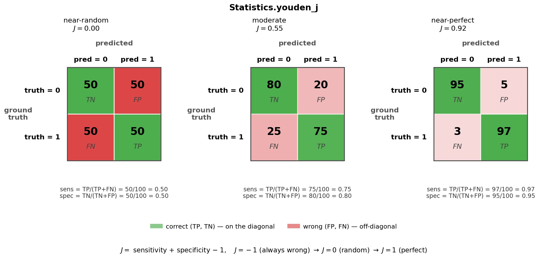
Parameters

• sample_1 – The first binary array (ground truth or reference).

• sample_2 – The second binary array (predictions or test results).

Returns

Youden’s J statistic. Returns NaN if either sensitivity or specificity cannot be calculated (division by zero).

Return type

float

References

1

Youden, W. J. (1950). Index for rating diagnostic tests. Cancer, 3(1), 32–35.

Example

>>> y_true = np.array([1, 1, 0, 0, 1, 0, 1, 1, 0, 0])
>>> y_pred = np.array([1, 1, 0, 1, 1, 0, 1, 0, 0, 0])
>>> j = Statistics.youden_j(sample_1=y_true, sample_2=y_pred)

static yule_coef(x, y, w=None)

Jitted calculate of the yule coefficient between two binary vectors (e.g., to classified behaviors). 0 represent independence, 2 represents complete interdependence.

\[Yule Coefficient = \frac{{2 \cdot t_f \cdot f_t}}{{t_t \cdot f_f + t_f \cdot f_t}}\]

Note

Adapted from pynndescent.

Parameters

• x (np.ndarray) – First binary vector.

• y (np.ndarray) – Second binary vector.

• w (Optional[np.ndarray]) – Optional weights for each element. Can be classification probabilities. If not provided, equal weights are assumed.

Returns

yule coefficient

Return type

float

Example

>>> x = np.random.randint(0, 2, (50,)).astype(np.int8)
>>> y = x ^ 1
>>> Statistics().yule_coef(x=x, y=y)
>>> 2
>>> random_indices = np.random.choice(len(x), size=len(x)//2, replace=False)
>>> y = np.copy(x)
>>> y[random_indices] = 1 - y[random_indices]
>>> Statistics().yule_coef(x=x, y=y)
>>> 0.99

Statistics GPU methods

simba.data_processors.cuda.statistics.adjusted_rand_gpu(x, y)

Calculate the Adjusted Rand Index (ARI) between two clusterings.

The Adjusted Rand Index (ARI) is a measure of the similarity between two clusterings. It considers all pairs of samples and counts pairs that are assigned to the same or different clusters in both the true and predicted clusterings.

The ARI is defined as:

\[ARI = \frac{TP + TN}{TP + FP + FN + TN}\]

where:

• \(TP\) (True Positive) is the number of pairs of elements that are in the same cluster in both x and y,

• \(FP\) (False Positive) is the number of pairs of elements that are in the same cluster in y but not in x,

• \(FN\) (False Negative) is the number of pairs of elements that are in the same cluster in x but not in y,

• \(TN\) (True Negative) is the number of pairs of elements that are in different clusters in both x and y.

The ARI value ranges from -1 to 1. A value of 1 indicates perfect clustering agreement, 0 indicates random clustering, and negative values indicate disagreement between the clusterings.

Note

Modified from scikit-learn

See also

For CPU call, see simba.mixins.statistics_mixin.Statistics.adjusted_rand().

Parameters

• x (np.ndarray) – 1D array representing the labels of the first model.

• y (np.ndarray) – 1D array representing the labels of the second model.

Returns

A value of 1 indicates perfect clustering agreement, a value of 0 indicates random clustering, and negative values indicate disagreement between the clusterings.

Return type

float

Example

>>> x = np.random.randint(low=0, high=55, size=100000000)
>>> y = np.random.randint(low=0, high=55, size=100000000)
>>> adjusted_rand_gpu(x=x, y=y)

simba.data_processors.cuda.statistics.count_values_in_ranges(x, r)

Counts the number of values in each feature within specified ranges for each row in a 2D array using CUDA.

EXPECTED RUNTIMES
FRAMES (MILLION)	TIME (S)
4	0.038
8	0.201
16	0.344
32	0.306
64	0.776
128	1.611
NVIDIA GeForce RTX 4070
(n, 11)

See also

For CPU function see count_values_in_range().

Parameters

• x (np.ndarray) – 2d array with feature values.

• r (np.ndarray) – 2d array with lower and upper boundaries.

Returns

2d array of size len(x) x len(r) with the counts of values in each feature range (inclusive).

Return type

np.ndarray

Example

>>> x = np.random.randint(1, 11, (10, 10)).astype(np.int8)
>>> r = np.array([[1, 6], [6, 11]])
>>> r_x = count_values_in_ranges(x=x, r=r)

simba.data_processors.cuda.statistics.davis_bouldin(x, y)

Computes the Davis-Bouldin Index using GPU acceleration, a clustering evaluation metric that assesses the quality of clustering based on the ratio of within-cluster and between-cluster distances.

The lower the Davis-Bouldin Index, the better the clusters are separated and compact. The function calculates the average similarity between each cluster and its most similar cluster.

See also

For CPU implementation, use simba.mixins.statistics_mixin.Statistics.davis_bouldin()

EXPECTED RUNTIMES
OBSERVATIONS (MILLIONS)	TIME (S)	STDEV (S)
2	0.03166	0.023
4	0.06161	0.04883
8	0.12143	0.09597
16	0.24169	0.19592
32	0.27942	0.12019
64	0.45187	0.09255
128	0.98631	0.31372
NVIDIA GeForce RTX 4070
REPEATS = 3
centers = [[0, 0], [5, 10], [10, 0], [20, 10]]
x, y = make_blobs(n_samples=OBSERVATIONS, n_features=2, centers=centers, cluster_std=1)

Parameters

• x (np.ndarray) – A 2D array of data points where each row corresponds to aan observation and each column corresponds to a feature.

• y (np.ndarray) – A 1D array containing the cluster labels for each sample in x.

Returns

The Davis-Bouldin Index as a float, where lower values indicate better-defined clusters.

Return type

float

Example

>>> centers = [[0, 0], [5, 10], [10, 0], [20, 10]]  # Adjust distances between cluster centers
>>> x, y = make_blobs(n_samples=50000, n_features=4, centers=3, cluster_std=0.1)
>>> p = davis_bouldin(x, y)

simba.data_processors.cuda.statistics.dunn_index(x, y)

Computes the Dunn Index for clustering quality using GPU acceleration, which is a ratio of the minimum inter-cluster distance to the maximum intra-cluster distance. The higher the Dunn Index, the better the separation between clusters.

The Dunn Index is given by:

\[D = \frac{\min_{i \neq j} \{ \delta(C_i, C_j) \}}{\max_k \{ \Delta(C_k) \}}\]

where \(\delta(C_i, C_j)\) is the distance between clusters \(C_i\) and \(C_j\), and \(\Delta(C_k)\) is the diameter of cluster \(C_k\).

The higher the Dunn Index, the better the clustering, as a higher value indicates that the clusters are well-separated relative to their internal cohesion.

EXPECTED RUNTIMES
OBSERVATIONS (MILLIONS)	TIME (S)	STDEV (S)
2	0.2366	0.0114
4	0.4464	0.0016
8	0.9037	0.0032
16	1.8675	0.0019
32	3.6247	0.006497
64	7.2898	0.007388
128	14.822	0.02672
256	29.316	0.0425
512	58.23599271	0.477388716
NVIDIA GeForce RTX 4070
REPEATS = 3
centers = [[0, 0], [5, 10], [10, 0], [20, 10]]
x, y = make_blobs(n_samples=OBSERVATIONS, n_features=2, centers=centers, cluster_std=1)

Parameters

• x (np.ndarray) – The input data points, where each row corresponds to an observation, and columns are features.

• y (np.ndarray) – Cluster labels for the data points. Each label corresponds to a cluster assignment for the respective observation in x.

Returns

The Dunn Index, a floating point value that measures the quality of clustering.

Return type

float

Example

>>> centers = [[0, 0], [5, 10], [10, 0], [20, 10]]  # Adjust distances between cluster centers
>>> x, y = make_blobs(n_samples=80_000_000, n_features=10, centers=centers, cluster_std=1, random_state=10)
>>> v = dunn_index(x=x, y=y)

simba.data_processors.cuda.statistics.euclidean_distance_to_static_point(data, point, pixels_per_millimeter=1, centimeter=False, batch_size=65000000)

Computes the Euclidean distance between each point in a given 2D array data and a static point using GPU acceleration.

See also

For CPU-based distance to static point (ROI center), see simba.mixins.feature_extraction_mixin.FeatureExtractionMixin.framewise_euclidean_distance_roi() For CPU-based framewise Euclidean distance, see simba.mixins.feature_extraction_mixin.FeatureExtractionMixin.framewise_euclidean_distance() For GPU CuPy solution for distance between two sets of points, see simba.data_processors.cuda.statistics.get_euclidean_distance_cupy() For GPU numba CUDA solution for distance between two sets of points, see simba.data_processors.cuda.statistics.get_euclidean_distance_cuda()

Parameters

• data – A 2D array of shape (N, 2), where N is the number of points, and each point is represented by its (x, y) coordinates. The array can represent pixel coordinates.

• point – A tuple of two integers representing the static point (x, y) in the same space as data.

• pixels_per_millimeter – A scaling factor that indicates how many pixels correspond to one millimeter. Defaults to 1 if no scaling is necessary.

• centimeter – A flag to indicate whether the output distances should be converted from millimeters to centimeters. If True, the result is divided by 10. Defaults to False (millimeters).

• batch_size – The number of points to process in each batch to avoid memory overflow on the GPU. The default batch size is set to 65 million points (6.5e+7). Adjust this parameter based on GPU memory capacity.

Returns

A 1D array of distances between each point in data and the static point, either in millimeters or centimeters depending on the centimeter flag.

Return type

np.ndarray

simba.data_processors.cuda.statistics.get_3pt_angle(x, y, z)

Computes the angle formed by three points in 2D space for each corresponding row in the input arrays using GPU. The points x, y, and z represent the coordinates of three points in space, and the angle is calculated at point y between the line segments xy and yz.

EXPECTED RUNTIMES
FRAMES	TIME (S)
4 million	0.02
8 million	0.04
16 million	0.159
32 million	0.29
64 million	0.335
128 million	0.792
256 million	1.371

See also

For CPU function see angle3pt() and For CPU function see angle3pt_serialized().

Parameters

• x – A numpy array of shape (n, 2) representing the first point (e.g., nose) coordinates.

• y – A numpy array of shape (n, 2) representing the second point (e.g., center) coordinates, where the angle is computed.

• z – A numpy array of shape (n, 2) representing the second point (e.g., center) coordinates, where the angle is computed.

Returns

A numpy array of shape (n, 1) containing the calculated angles (in degrees) for each row.

Return type

np.ndarray

Example

>>> video_path = r"/mnt/c/troubleshooting/mitra/project_folder/videos/501_MA142_Gi_CNO_0514.mp4"
>>> data_path = r"/mnt/c/troubleshooting/mitra/project_folder/csv/outlier_corrected_movement_location/501_MA142_Gi_CNO_0514 - test.csv"
>>> df = read_df(file_path=data_path, file_type='csv')
>>> y = df[['Center_x', 'Center_y']].values
>>> x = df[['Nose_x', 'Nose_y']].values
>>> z = df[['Tail_base_x', 'Tail_base_y']].values
>>> angle_x = get_3pt_angle(x=x, y=y, z=z)

simba.data_processors.cuda.statistics.get_euclidean_distance_cuda(x, y)

Computes the Euclidean distance between two sets of points using CUDA for GPU acceleration.

EXPECTED RUNTIMES
OBSERVATION	TIME (S)
110k	0.007
181k	0.021
327k	0.032
620k	0.02
1.2m	0.082
2.4m	0.046
4.7m	0.106
9.3m	0.209
18.6m	0.238
37.2m	0.926
74.5m	1.136
149m	2.046

See also

For CPU function see framewise_euclidean_distance(). For CuPY function see get_euclidean_distance_cupy().

Parameters

• x (np.ndarray) – A 2D array of shape (n, m) representing n points in m-dimensional space. Each row corresponds to a point.

• y (np.ndarray) – A 2D array of shape (n, m) representing n points in m-dimensional space. Each row corresponds to a point.

Return np.ndarray

A 1D array of shape (n,) where each element represents the Euclidean distance between the corresponding points in x and y.

Example

>>> video_path = r"/mnt/c/troubleshooting/mitra/project_folder/videos/501_MA142_Gi_CNO_0514.mp4"
>>> data_path = r"/mnt/c/troubleshooting/mitra/project_folder/csv/outlier_corrected_movement_location/501_MA142_Gi_CNO_0514 - test.csv"
>>> df = read_df(file_path=data_path, file_type='csv')[['Center_x', 'Center_y']]
>>> shifted_df = FeatureExtractionMixin.create_shifted_df(df=df, periods=1)
>>> x = shifted_df[['Center_x', 'Center_y']].values
>>> y = shifted_df[['Center_x_shifted', 'Center_y_shifted']].values
>>> get_euclidean_distance_cuda(x=x, y=y)

simba.data_processors.cuda.statistics.get_euclidean_distance_cupy(x, y, batch_size=35000000007)

Computes the Euclidean distance between corresponding pairs of points in two 2D arrays using CuPy for GPU acceleration. The computation is performed in batches to handle large datasets efficiently.

See also

For CPU function see framewise_euclidean_distance(). For CUDA JIT function see get_euclidean_distance_cuda().

Parameters

• x (np.ndarray) – A 2D NumPy array with shape (n, 2), where each row represents a point in a 2D space.

• y (np.ndarray) – A 2D NumPy array with shape (n, 2), where each row represents a point in a 2D space. The shape of y must match the shape of x.

• batch_size (Optional[int]) – The number of points to process in a single batch. This parameter controls memory usage and can be adjusted based on available GPU memory. The default value is large (3.5e10 + 7) to maximize GPU utilization, but it can be lowered if memory issues arise.

Returns

A 1D NumPy array of shape (n,) containing the Euclidean distances between corresponding points in x and y.

Return type

np.ndarray

Example

>>> x = np.array([[1, 2], [3, 4], [5, 6]])
>>> y = np.array([[7, 8], [9, 10], [11, 12]])
>>> distances = get_euclidean_distance_cupy(x, y)

simba.data_processors.cuda.statistics.hamming_distance_gpu(x, y, w=None)

Computes the weighted Hamming distance between two arrays using GPU acceleration.

EXPECTED RUNTIMES
OBSERVATIONS (COUNT)	GPU TIME (S) (NUMBA CUDA)	CPU TIME (S) (NUMBA NJIT)
10k	0.01209025	0.00057592
100k	0.00364709	0.00553586
1m	0.0223	0.0551
10m	0.152	0.771
100m	0.4393	5.858
250m	1.3283	14.8490987
500m	2.2082	29.562
1tn	4.821	59.8388138
NVIDIA GeForce RTX 4070, 32 CORES

See also

For jitted CPU method, see simba.mixins.statistics_mixin.Statistics.hamming_distance().

Parameters

• x (ndarray) – A 1D or 2D NumPy array representing the reference data. If 2D, shape should be (n_samples, n_features). Supported dtypes are numeric.

• y (ndarray) – Array of the same shape as x representing the data to compare.

• w (ndarray) – A 1D array of shape (n_samples,) representing sample weights. If None, uniform weights are used.

Returns

The weighted average Hamming distance between corresponding rows of x and y.

Return type

float

Example

>>> x, y = np.random.randint(0, 2, (10, 1)).astype(np.int8), np.random.randint(0, 2, (10, 1)).astype(np.int8)
>>> gpu_hamming = hamming_distance_gpu(x=x, y=y)

simba.data_processors.cuda.statistics.i_index(x, y, verbose=False)

Calculate the I-Index for evaluating clustering quality.

The I-Index is a metric that measures the compactness and separation of clusters. A higher I-Index indicates better clustering with compact and well-separated clusters.

EXPECTED RUNTIMES
OBSERVATIONS (MILLIONS)	TIME (S)	STD TIME(S)
5	1.501366667	0.096872717
10	3.0527	0.117796944
20	5.9634	0.282048418
40	11.44683333	0.087952051
80	22.74773333	0.110135477
160	49.425	0.420928735
NVIDIA GeForce RTX 4070
7 body-parts
100 clusters / 3 features

The I-Index is calculated as:

\[I = \frac{SST}{k \times SWC}\]

where:

• \(SST = \sum_{i=1}^{n} \|x_i - \mu\|^2\) is the total sum of squares (sum of squared distances from all points to the global centroid)

• \(k\) is the number of clusters

• \(SWC = \sum_{c=1}^{k} \sum_{i \in c} \|x_i - \mu_c\|^2\) is the within-cluster sum of squares (sum of squared distances from points to their cluster centroids)

See also

To compute Xie-Beni on the CPU, use i_index()

Parameters

• x (np.ndarray) – The dataset as a 2D NumPy array of shape (n_samples, n_features).

• y (np.ndarray) – Cluster labels for each data point as a 1D NumPy array of shape (n_samples,).

Returns

The I-index score for the dataset.

Return type

float

References

1

Zhao, Q., Xu, M., & Fränti, P. (2009). Sum-of-squares based cluster validity index and significance analysis. In Adaptive and Natural Computing Algorithms (ICANNGA 2009), Lecture Notes in Computer Science, vol. 5495. Springer.

Example

>>> X, y = make_blobs(n_samples=5000, centers=20, n_features=3, random_state=0, cluster_std=0.1)
>>> i_index(x=X, y=y)

simba.data_processors.cuda.statistics.kmeans_cuml(data, k=2, max_iter=300, output_type=None, sample_n=None)

CRAP, SLOWER THAN SCIKIT

simba.data_processors.cuda.statistics.kullback_leibler_divergence_gpu(x, y, fill_value=1, bucket_method='scott', verbose=False)

Compute Kullback-Leibler divergence between two distributions.

Note

Empty bins (0 observations in bin) in is replaced with passed fill_value.

Its range is from 0 to positive infinity. When the KL divergence is zero, it indicates that the two distributions are identical. As the KL divergence increases, it signifies an increasing difference between the distributions.

See also

For CPU implementation, see simba.mixins.statistics_mixin.Statistics.kullback_leibler_divergence().

Parameters

• x (ndarray) – First 1d array representing feature values.

• y (ndarray) – Second 1d array representing feature values.

• fill_value (Optional[int]) – Optional pseudo-value to use to fill empty buckets in y histogram

• bucket_method (Literal) – Estimator determining optimal bucket count and bucket width. Default: The maximum of the Sturges and Freedman-Diaconis estimators

Returns

Kullback-Leibler divergence between x and y

Return type

float

Example

>>> x, y = np.random.normal(loc=150, scale=900, size=10000000), np.random.normal(loc=140, scale=900, size=10000000)
>>> kl = kullback_leibler_divergence_gpu(x=x, y=y)

simba.data_processors.cuda.statistics.silhouette_score_gpu(x, y, metric='euclidean')

Compute the Silhouette Score for clustering assignments on GPU using a specified distance metric.

Parameters

• x (np.ndarray) – Feature matrix of shape (n_samples, n_features) containing numeric data.

• y (np.ndarray) – Cluster labels array of shape (n_samples,) with numeric labels.

• metric (Literal["cityblock", "cosine", "euclidean", "l1", "l2", "manhattan", "sqeuclidean"]) – Distance metric to use (default=’euclidean’). Must be one of: “cityblock”, “cosine”, “euclidean”, “l1”, “l2”, “manhattan”, or “sqeuclidean”.

Returns

Mean silhouette score as a float.

Return type

float

Example

>>> x, y = make_blobs(n_samples=50000, n_features=20, centers=5, cluster_std=10, center_box=(-1, 1))
>>> score_gpu = silhouette_score_gpu(x=x, y=y)

simba.data_processors.cuda.statistics.sliding_mean(x, time_window, sample_rate)

Computes the mean of values within a sliding window over a 1D numpy array x using CUDA for acceleration.

EXPECTED RUNTIMES
FRAMES (MILLIONS)	TIME (S)
2	0.005
4	0.025
8	0.015
16	0.028
32	0.059
64	0.182
128	0.237
256	0.507
512	1.022
NVIDIA GeForce RTX 4070
time window = 1s / 10 FPS

Parameters

• x (np.ndarray) – The input 1D numpy array of floats. The array over which the sliding window sum is computed.

• time_window (float) – The size of the sliding window in seconds. This window slides over the array x to compute the sum.

• sample_rate (int) – The number of samples per second in the array x. This is used to convert the time-based window size into the number of samples.

Returns

A numpy array containing the sum of values within each position of the sliding window.

Return type

np.ndarray

Example

>>> x = np.random.randint(1, 11, (100, )).astype(np.float32)
>>> time_window = 1
>>> sample_rate = 10
>>> r_x = sliding_mean(x=x, time_window=time_window, sample_rate=10)

simba.data_processors.cuda.statistics.sliding_min(x, time_window, sample_rate)

Computes the minimum value within a sliding window over a 1D numpy array x using CUDA for acceleration.

EXPECTED RUNTIMES
FRAMES (MILLIONS)	TIME (S)
2	0.003
4	0.016
8	0.012
16	0.049
32	0.053
64	0.099
128	0.211
256	0.495
512	1.031
NVIDIA GeForce RTX 4070
time window = 1s / 10 FPS

Parameters

• x (np.ndarray) – Input 1D numpy array of floats. The array over which the sliding window minimum is computed.

• time_window (float) – The size of the sliding window in seconds.

• sample_rate (int) – The sampling rate of the data, which determines the number of samples per second.

Returns

A numpy array containing the minimum value for each position of the sliding window.

Return type

np.ndarray

Example

>>> x = np.arange(0, 10000000)
>>> time_window = 1
>>> sample_rate = 10
>>> sliding_min(x=x, time_window=time_window, sample_rate=sample_rate)

simba.data_processors.cuda.statistics.sliding_spearmans_rank(x, y, time_window, sample_rate, batch_size=16000000, verbose=False)

Computes the Spearman’s rank correlation coefficient between two 1D arrays x and y over sliding windows of size time_window * sample_rate. The computation is performed in batches to optimize memory usage, leveraging GPU acceleration with CuPy.

See also

For CPU function see sliding_spearman_rank_correlation().

\(\rho = 1 - \frac{6 \sum d_i^2}{n_w(n_w^2 - 1)}\)

Where: - \(\rho\) is the Spearman’s rank correlation coefficient. - \(d_i\) is the difference between the ranks of corresponding elements in the sliding window. - \(n_w\) is the size of the sliding window.

Parameters

• x (np.ndarray) – The first 1D array containing the values for Feature 1.

• y (np.ndarray) – The second 1D array containing the values for Feature 2.

• time_window (float) – The size of the sliding window in seconds.

• sample_rate (int) – The sampling rate (samples per second) of the data.

• batch_size (Optional[int]) – The size of each batch to process at a time for memory efficiency. Defaults to 1.6e7.

Returns

A 1D numpy array containing the Spearman’s rank correlation coefficient for each sliding window.

Return type

np.ndarray

Example

>>> x = np.array([9, 10, 13, 22, 15, 18, 15, 19, 32, 11])
>>> y = np.array([11, 12, 15, 19, 21, 26, 19, 20, 22, 19])
>>> sliding_spearmans_rank(x, y, time_window=0.5, sample_rate=2)

simba.data_processors.cuda.statistics.sliding_std(x, time_window, sample_rate)

Parameters

• x (np.ndarray) – The input 1D numpy array of floats. The array over which the sliding window sum is computed.

• time_window (float) – The size of the sliding window in seconds. This window slides over the array x to compute the sum.

• sample_rate (int) – The number of samples per second in the array x. This is used to convert the time-based window size into the number of samples.

Returns

A numpy array containing the sum of values within each position of the sliding window.

Return type

np.ndarray

Example

>>> x = np.random.randint(1, 11, (100, )).astype(np.float32)
>>> time_window = 1
>>> sample_rate = 10
>>> r_x = sliding_sum(x=x, time_window=time_window, sample_rate=10)

simba.data_processors.cuda.statistics.sliding_sum(x, time_window, sample_rate)

Computes the sum of values within a sliding window over a 1D numpy array x using CUDA for acceleration.

Parameters

• x (np.ndarray) – The input 1D numpy array of floats. The array over which the sliding window sum is computed.

• time_window (float) – The size of the sliding window in seconds. This window slides over the array x to compute the sum.

• sample_rate (int) – The number of samples per second in the array x. This is used to convert the time-based window size into the number of samples.

Returns

A numpy array containing the sum of values within each position of the sliding window.

Return type

np.ndarray

Example

>>> x = np.random.randint(1, 11, (100, )).astype(np.float32)
>>> time_window = 1
>>> sample_rate = 10
>>> r_x = sliding_sum(x=x, time_window=time_window, sample_rate=10)

simba.data_processors.cuda.statistics.sokal_sneath_gpu(x, y, w=None)

Compute the Sokal–Sneath similarity coefficient between two binary vectors using CUDA acceleration.

See also

For CPU method, see simba.mixins.statistics_mixin.Statistics.sokal_sneath()

Parameters

• x (ndarray) – First binary vector (1D array of 0s and 1s).

• y (ndarray) – Second binary vector of the same shape as x.

• w (ndarray) – A 1D array of shape (n_samples,) representing sample weights. If None, uniform weights are used.

Returns

The Sokal–Sneath similarity coefficient between x and y.

Return type

float.

simba.data_processors.cuda.statistics.xie_beni(x, y)

Computes the Xie-Beni index for clustering evaluation.

The score is calculated as the ratio between the average intra-cluster variance and the squared minimum distance between cluster centroids. This ensures that the index penalizes both loosely packed clusters and clusters that are too close to each other.

A lower Xie-Beni index indicates better clustering quality, signifying well-separated and compact clusters.

See also

To compute Xie-Beni on the CPU, use xie_beni() Significant GPU savings detected at about 1m features, 25 clusters.

Parameters

• x (np.ndarray) – The dataset as a 2D NumPy array of shape (n_samples, n_features).

• y (np.ndarray) – Cluster labels for each data point as a 1D NumPy array of shape (n_samples,).

Returns

The Xie-Beni score for the dataset.

Return type

float

Example

>>> from sklearn.datasets import make_blobs
>>> X, y = make_blobs(n_samples=100000, centers=40, n_features=600, random_state=0, cluster_std=0.3)
>>> xie_beni(x=X, y=y)

References

1

Xie, X. L., & Beni, G. (1991). A validity measure for fuzzy clustering. IEEE Transactions on Pattern Analysis and Machine Intelligence, 13(8), 841–847.